iLOV Characterisation

The aim of this study is threefold: the emmission spectra of iLOV will be explored over a range of excitation wavelengths, recovery rates from photo bleaching will be measured and iLOV's performance in low oxygen environments will be characterised.

Prior to selecting explosive degrading genes, a reporter gene that would enable quick feedback on the successful expression of operons was needed. The reporter gene would also be used in a biosensor of explosive compounds. While the Green Fluorescent Protein (GFP) and its variants are the most commonly used reporters on the iGEM database and in the wider scientific community, the protein iLOV was chosen as the reporter for our constructs.

iLOV was introduced to the iGEM database in 2011 by Glasgow University \cite{Glasgow}, but so far has seen no further characterization. iLOV has a range of advantages over GFP and related florescent proteins (FP) including:

Ability to work in anoxic conditions \cite{Glasgow}
Recovers spontaneously after photo-bleaching \cite{Chapman}
Shorter sequence than GFP \cite{Chapman}
Faster maturation of iLOV flurophore than GFP \cite{Chapman}
Stable over a wide pH range \cite{Swartz}

iLOV's pH compatibility and photo-bleaching resistance are crucial to the success of a biosensor device that would be required to work in a range of soil types and climates. For example some of the most heavily mine contaminated areas in the world are in western Sahara along the Berm, a 1500 mile long minefield built to protect the Morrocan border. Under such conditions an on-site application of the bio-sensor would need to resist photo bleaching in the harsh Saharan sunlight.

iLOV's ability to work in anoxic conditions will allow it to work in heavily contaminated water supplies such as those from mining sites where eutrophication, caused by leaching from the site, has occurred.

Experimental Method

Excitation and Emission Scanning

The scanning of the excitation and emission spectra would occur in two stages. First a broad range scan, 5nm spacing between emission scans, would give the general topography of florescence from the iLOV protein. Then the areas around the peaks from the broad range scan would be explored more throughly with 1nm spaced emission scans.

The scans would be made using a TECAN florescence measuring machine. This machine is capable of measuring fluorescence across a 96 well plate, enabling multiple measurements of each iLOV growth culture. The pitfall of the machine's high through put design is that measurements of fluorescence are made by both exciting the protein and detecting emitted photons along the same axis (Directly above the well). This results in photons emitted from the machine reflecting back from the bottom of the well and interfering in emission measurements. As such the TECAN cannot measure emissions from the protein that are closer than about 30nm from excitation wavelengths.

The iLOV protein would be scanned in-vivo inside a Top 10 strain of cells. A control Top 10 culture would also be scanned and the difference in fluorescence would be taken as the emission profile of iLOV. The Top 10 strain cells (With and without the iLOV expression plasmid) where grown up overnight in liquid broth before 10$\mu$l of the culture was added to 190$\mu$l of minimal media into each well of the 96 well plate.

Minimal media was used to remove the systematic error that would have been caused by the autofluorescence of normal Lysogeny Broth (LB).

Twelve wells of the 96 well plate were filled with each of the cultures. The cultures where grown at 37$^{\circ}$C whilst being rotated at 800rpm to allow air into the media until they reached an optical density (OD) above 0.5 at 600nm.

Once the required OD was reached the emission scans began. First the Broad range emission scans at excitation intervals of 5nm from 350nm to 500nm were made, emission was measured from 400nm to 700nm in 5nm intervals. To reduce the systematic error introduced by photo-bleaching the protein the number of emission reads for each measurement was limited to five. Due to reflection from the excitation photons a portion of the measurements must be discounted where the excitation wavelength came within around 30nm of the emission measurement wavelength.

To find the peaks of iLOV fluorescence the fluorescence from each well was divided by the OD in that well to give the relative fluorescence per cell. The relative fluorescence of the control Top 10 cells was then subtracted from those Top 10 cells with the iLOV plasmid.

The second set, of finer spaced emission scans, were then carried out about the peak(s). These scans were taken at 1nm excitation and emission intervals between points defined by the prior part of this experiment.

To try and prevent photo bleaching of the iLOV protein only three wells where used for each set of measurements. The set of wells used was alternated over the course of the experiment. For the finer spaced measurements six well where used to improve the accuracy of the result.

Results, Analysis and discussion

Excitation and Emission Scanning

The fluorescence from the iLOV protein is found using equation \ref{Fluor},

The fluorescence from each of the wells is divided by the OD in that well ($O_{i/j}$). The average fluorescence per OD of the Top 10 cells ($g_j$) is then subtracted from the average fluorescence per OD of the Top 10 cells with iLOV expressing sequences ($f_i$). This should leave only the fluorescence due to the iLOV protein.

Figure \ref{Broad} shows the emission topography of the iLOV protein in E.coli. It is clear that there is one large peak of emission centered around an excitation wavelength of 440nm which causes the iLOV protein to emit at around 500nm. The plane of zero fluorescence at the top left of figure \ref{Broad} is caused by reflection from the excitation photons.

Following from this result the area between 420nm and 480nm excitation wavelengths were chosen to be scanned at a higher resolution. The emitted fluorescence would be measured at 2nm intervals between 460nm and 550nm for excitation wavelengths spaced 1nm apart.

Figure \ref{Ridged} shows the result of the higher resolution scan. It can immediately be seen that there is some artificial effect at work. The striation of the results is most probably caused by photo bleaching, where the exciting photons have changed the conformation of the protein. The altered state of the protein may have a higher or lower rate of reemission of the excitation photons.

The striation of the results invalidates them from determining the peak emission and excitation wavelength as it cannot be determined whether it is the rest conformation of iLOV that is being measured.

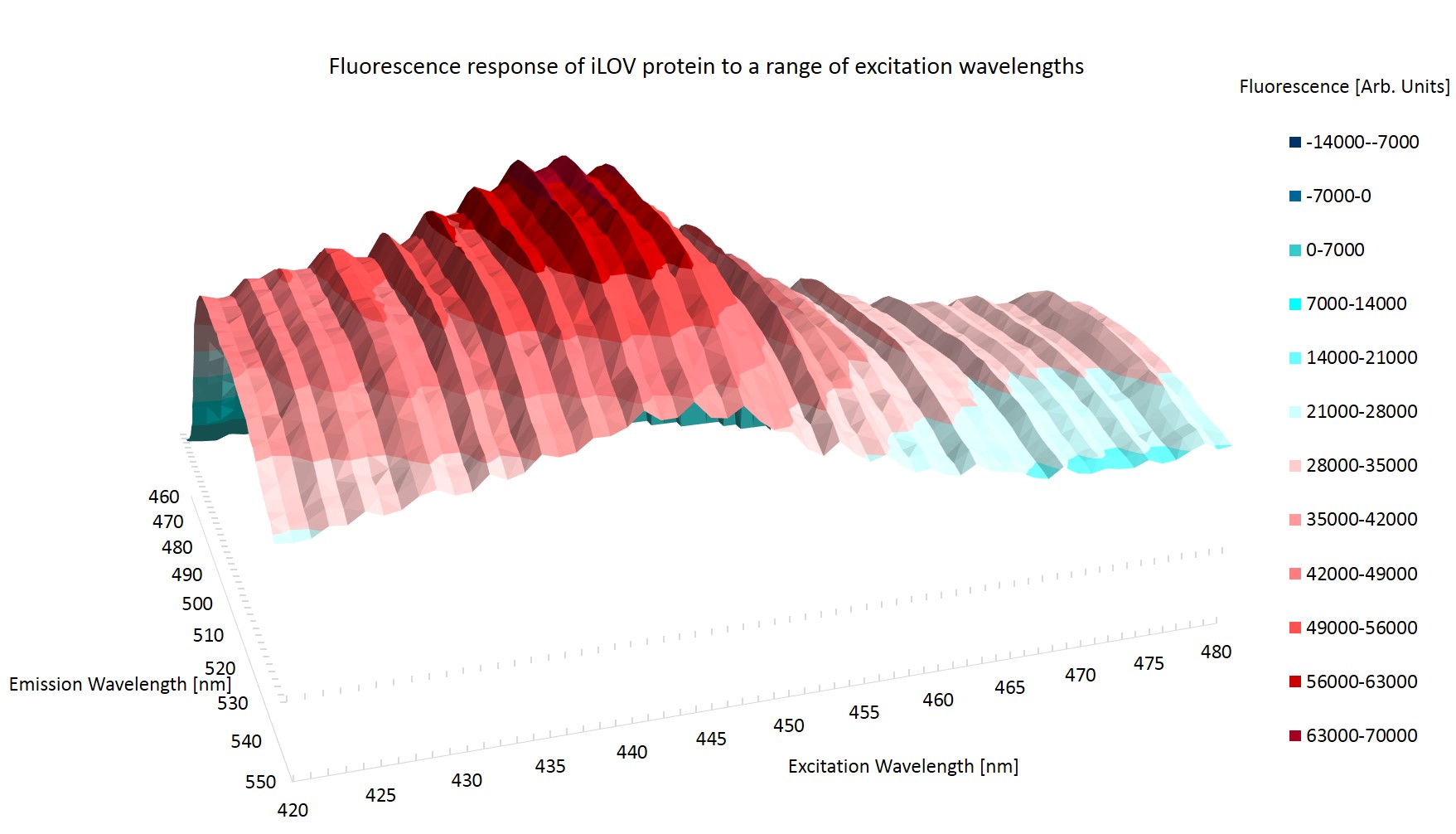
Photo bleaching was observed in the high resolution scan but not in the broad range scan. This may be because during the broad range emission scans the proteins are exposed to exciting photons for 1.8 ms per scan, whilst in the high resolution scan the protein are exposed for 4.5ms per scan. Three scans are taken in quick succession.

To try and determine whether the effect is indeed artificial, the fluorescence emission at 500nm was plotted across the excitation wavelengths. This can be seen in figure \ref{Striated}. The triplets of successive scans are coloured. This was done to see if any pattern might become apparent. Measurements taken from the the broad range scan are also plotted for reference.

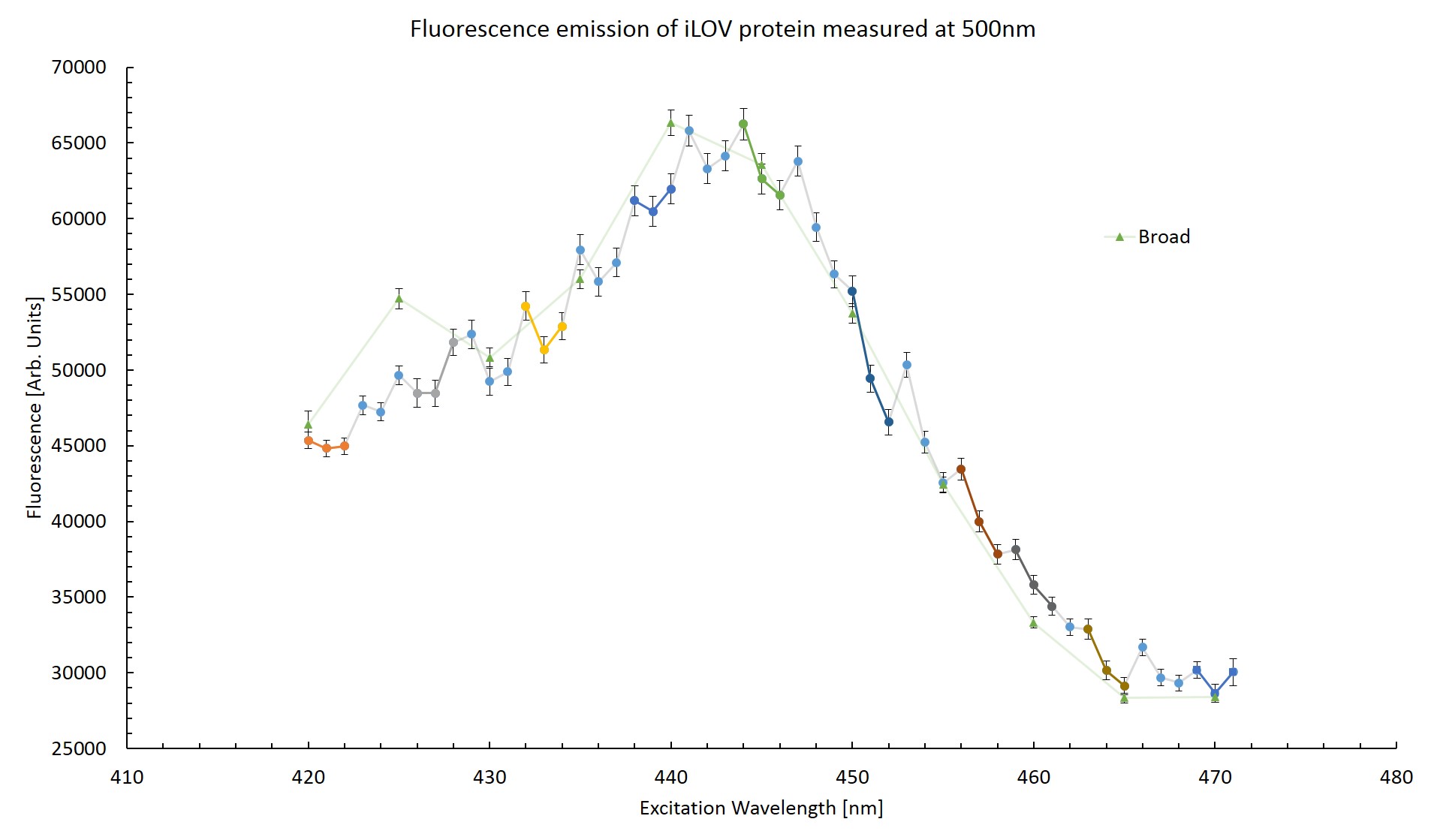
From figure \ref{Striated} it can be seen that the first measurement is notably higher than the trend for the next two measurements in each triplet. This would suggest that the protein has been photo-bleached as the emission response decrease after exposure to excitation photons. The difference in fluorescence between the high resolution scan and the broad range scan is greatest at excitation wavelengths of 420nm and 440nm which correspond to measurements taken in the final scan of a triplet. Too few measurements can be compared to make any conclusion based off this plot. This effect will be explored in more detail in section \ref{Bleach}.

The errors in figure \ref{Striated} are calculated via equation \ref{Error},

\begin{equation} \delta F = \sqrt{\sum_{i}^{N}\left(\frac{f_i\delta O_i}{O_i^2 N}\right)^2+\sum_{j}^{M}\left(\frac{g_j\delta O_j}{O_j^2 M}\right)^2}, \label{Error} \end{equation}

where $\delta O_i$ is the error in the OD for each well, $f_i$, $g_i$ are the fluorescence measurements from iLOV and Top 10 wells respectively and N, M are the number of wells used.

Due to the striation of the fine-scale results a previous measurement was used to confirm the peak of fluorescence. This result can be seen in figure \ref{LB}. This result was not used originally as measurements where carried out in Lysogeny Broth (LB) which has a higher autofluorescence than the minimal media used previously. The higher autofluorescence of the LB resulted in a masking of the fluorescence topography from the Top 10 wells. This resulted in the Top 10 cells without iLOV sequences reading as having a higher fluorescence than those with the iLOV sequence for certain ares of the experimental space. The fluorescence topography of the iLOV protein is still visible despite this and matches the topography observed in minimal media.

The peak excitation wavelength is 449$\pm$1 nm and the peak emission corresponding to this excitation wavelength is 494$\pm$2nm. The peak has a lower apparent fluorescence than previous measurements, this is due to a lower manual gain on these measurements. The manual gain is the factor that the measured intensity is multiplied by. It was lowered for these measurements in an effort to take emission measurements closer to the excitation wavelength. However this was unsuccessful, only resulting in some reflection measurements being read as within the acceptable fluorescence range.

No photo bleaching is observed in this measurement despite the protein being exposed for 5ms per scan. This is likely due to the greater opacity of LB in comparison to minimal media.

\section{Conclusion}

\subsection{Excitation and Emission Scanning}

\begin{thebibliography}{9} \bibitem{Glasgow} 2011.igem.org/Team:Glasgow/LOV2 \bibitem{Chapman} The phtoreversible fluorescent protein iLOV outperforms GFP as a reporter of plant virus infection. Chapman, et al. www.png.org/content/105/50/20038.full \bibitem{Swartz} Swartz TE, et al. (2001) The photocycle of a flavin-binding domain of the blue light photoreceptor phototropin. \end{thebibliography}

Exeter | ERASE

Team:Exeter/iLOVCharacterisation

From 2014.igem.org

Contents

iLOV Characterisation

Experimental Method

Excitation and Emission Scanning

Results, Analysis and discussion

Excitation and Emission Scanning