From 2014.igem.org

Exeter | ERASE

Project Design

Biological modelling has been used for a variety of purposes. In this project we sought to build a model which would help us to design, analyse and debug our biological system . Furthermore, we wanted a method of visualising and explaining how our bacterium was performing. Specifically, our aims were:

The model should inform the biological design.
The model should inform the choice of experiments.
The model should be receptive to empirical observations.
The model should help explain how our biological system works.

Many iGEM teams have modelled their bacteria at the biochemical level using systems of differential equations. We started in the same manner, and then built a stochastic model on top of this to make the simulation more realistic. We then created a model of the diffusion of TNT across the cell membrane. Another model was created for the growth of the bacteria and the inclusion of a kill switch. Finally, we tried to bring these models together to create as accurate a model of our system as possible.

The Biochemical Level

We reasoned that the primary determinant of TNT degradation within the cell would be the activity of the introduced enzyme, either XenB or NemA (see Old Yellow Enzymes). The degradation of the TNT by these enzymes can be modelled by Michaelis-Menten kinetics. The most basic set of ordinary differential equations which would describe the system would be:

\begin{equation} \frac{d[\text{Cell}]}{dt}=g[\text{Cell}]−d[\text{TNT}] \end{equation} \begin{equation} \frac{d[TNT]}{dt}= \frac{−V_{\text{max}}\text{TNT}[\text{Cell}]}{K_m+ [\text{TNT}]} \end{equation}

where:

[$\text{Cell}$] is the number of cells in the colony.
[$\text{TNT}$] is the number of TNT molecules.
$g$ is the growth rate of the cells
$d$ is the rate at which TNT kills the cells.
$V_{\text{max}}$, $k_m$ are constants of the Michaelis-Menten equations.

In this model the concentration of enzyme is directly proportional to the number of cells. The cells grow at a rate $g$ and are destroyed at a rate proportional to the concentration of TNT in the system. The cells degrade the TNT according to Michaelis-Menten kinetics.

$V_{\text{max}}$ describes the maximum rate of reaction between the enzyme ([$\text{Cell}$]) and TNT. $K_m$ is the concentration at which half the maximum rate of degradation is achieved.

Data for the $k_{\text{cat}}$ and $K_m$ of XenB and NemA was not available, and so we initially ran the simulation using different arbitrary values. These yielded different distinct cases depending on the initial conditions. When the TNT was started at '20', and the amount of cells was started at '5', then the cells would ‘die out’. However, if the amount of cells was started at '10', and TNT remained at '20', the cell densitywould increase indefinitely and the amount of TNT would be reduced to 0. Therefore we have considered the cell density when applying our construct to a contaminted area.

In order to make this model more accurate it was necessary to gain information about the kinetics of XenB and NemA. We therefore sought to express recombinant XenB and NemA in E. coli, purify the proteins using a His-tag and determine the Kcat and Km directly. The results of this in vitro experimentation can be found in the sections Enzyme Kinetics: HPLC and Enzyme Kinetics: Raman.

The Cellular Level

Another primary determinant of TNT degradation rate will be the concentration of the substrate (TNT) within the cell. The concentration of TNT will be determined partly by the activity of XenB or NemA (see above) but also by the rate of diffusion of the TNT across the cell membrane. We therefore introduced a new set of equations:

\begin{equation} \frac{d[\text{Cell}]}{dt}=g[\text{Cell}]−d[\text{TNT}_{\text{in}}] \end{equation} \begin{equation} \frac{𝑑[\text{TNT}_{\text{in}}]}{dt}= −\frac{V_{\text{max}}\text{TNT}_{\text{in}}[\text{Cell}]}{K_m + \text{TNT}_{\text{in}}} + m \end{equation} \begin{equation} \frac{𝑑[\text{TNT}_{\text{out}}]}{dt}= −m \end{equation} \begin{equation} m \propto [\text{TNT}][\text{Cell}] \end{equation}

where:

$[\text{Cell}]$ is the number of cells in the colony.
$[\text{TNT}]$ is the number of TNT molecules.
$[\text{TNT}_{\text{in}}]$ is the number of TNT molecules inside cells.
$[\text{TNT}_{\text{out}}]$ is the number of TNT molecules outside cells.
$g$ is the growth rate of the cells.
$d$ is the rate at which TNT kills the cells.
$V_{\text{max}}$ and $k_m$ are constants of the Michaelis-Menten equations.
$m$ represents transport rate across the cell membrane.

This system, along with some arbitrary constants, was programmed into Matlab and the ode45 nonstiff differential equation solver gave results of the following form:

Figure 2: [Cell] was called [XenB] in the simulation.

According to this model, the amount of TNT in the system decreases over time. However, as with our first model, we do not know how well TNT crosses the cell membrane, i.e. the value for $m$ is unknown. We therefore sought to estimate diffusion rates ($m$) into the cell using Raman spectroscopy. The results can be seen here Enzyme Kinetics: Raman.

It is possible to add more and more elements to our system of differential equations; for example, the rate of transcription and translation of enzymes within the cell could be added. However, this would have only added more unknown coefficients to our equations. As such we decided to stop adding terms here as we were confident that values could be experimentally determined for each of the coefficients in the system.

At the time that the model was created the plan was that coefficients would be sourced from the following experiments:

Coefficient	Experiment
$g$, $d$	The Toxicity of TNT and Nitroglycerin to E. coli.
$V_{\text{max}}$, $k_m$	Validation of Enzyme Function and Activity
$m$	in vivo Activity

A Stochastic Model

Despite making the model more sophisticated, this remains a naive method of modelling the system. Fundamentally, the system of differential equations is designed so that it behaves as we would expect, and, as with any model, many assumptions are made. The system may not be accurately described by Michaelis-Menten kinetics. It is assumed, for example, that the cells and the TNT are completely mixed and there is no notion of the possibility of spatially variable concentration levels. We also assume that the amount of cells and TNT would be continuous, but in reality both the number of cells and the number of TNT molecules would be integers.

In order to address the problem of the number of cells not being continuous, we created a computer simulation that modelled a population of cells. The program simulated the state of the population over a certain amount of time, split into a number of time intervals.

At each interval, there was a constant probability of each cell splitting. When this happens, the concentrations of the substances inside the cells divide equally between the two cells. The cells could also die at each interval with a constant probability. If this happened, the substances would be distributed evenly across the other cells in the population.

Figure 3: Stochastic model, computationally intensive.

The results of this model were described by a list of parameters that corresponded to the constants (e.g. K_cat, K_m) in the differential equations. By adjusting these parameters different outcomes could be obtained. We ran the simulation with various values of $V_{\text{max}}$ and this showed that TNT was degraded faster at higher values (this would probably show a figure even if it is showing the same result as the simpler model). However, it should be noted that this result was clear from the initial equations. Our new model has not provided us with any new information at this point. However, this approach can be used as the basis for more complex models, and so we decided to introduce additional information in the form of the location of each cell in space.

Simulating diffusion across the phospholipid membrane

A major problem universal to synthetic biology is determining a method of bringing together products produced by the cell and the target of that product. One of the barriers to the movement of products produced by the cell is the phospholipid membrane. Many proteins are too large to cross this barrier without the help of membrane pumps. However, smaller molecules can move relatively freely across the boundary.

This model will attempt to determine whether our enzymes or TNT can freely move across the membrane. The time scales associated with this transport will also be ascertained. It will help us decide whether membrane pumps are also needed to to make our construct an effective method of degrading TNT.

The movement of smaller molecules across the lipid bi layer is largely governed by diffusion. Fick's law of diffusion can be used to describe the movement of TNT concentrations in a homogenous fluid:

\begin{equation} J=-DA \frac{dC}{dx}. \end{equation}

$J$ is the flux of particles over time (Also written as $\frac{dM}{dt}$ where $M$ is the mass of molecules). $\frac{dC}{dx}$ is the concentration gradient. $D$ is the diffusivity, the constant of proportionality between the molecule flux and the concentration gradient. $A$ is the area through which the molecules are moving.

If a distinction is made for a volume then this equation can be linearised (i.e. the differential is replaced with the difference in concentration inside $C_{\text{in}}$ and outside $C_{\text{out}}$ of that volume all divided by the length between the concentration measurements):

\begin{equation} J_m=-D_m A \frac{C_{\text{out}}-C_{\text{in}}}{l_m}. \end{equation}

This only holds true if the volume to which your molecules are moving has the same properties as that from where they came. For instance, if the molecule were moving into a membrane, then the molecules may be more soluble inside the membrane, and this will affect the rate of diffusion.

To take into account the difference in solubility between the two volumes we introduce a new quantity called the partition coefficient. It is defined as the ratio of concentrations at either side of a boundary:

\begin{equation} \beta = \frac{C_{\text{Inside}}}{C_{\text{Outside}}} \end{equation}

Applying this to the lipid bi-layer, $\beta$ is the partition coefficient between water and the lipids. We can extend this to create a system of ordinary differential equations to describe the movement of molecules across the membranes:

\begin{equation} \frac{d\text{TNT}_1}{dt}=-P_a (C_4-C_1), \end{equation} \begin{equation} \frac{d\text{TNT}_4}{dt}=P_a (C_4-C_1 )-P_b (C_5-C_4), \end{equation} \begin{equation} \frac{d\text{TNT}_5}{dt}=P_b (C_5-C_4 )-P_c (C_8-C_5), \end{equation} \begin{equation} \frac{d\text{TNT}_8}{dt}=P_c (C_8-C_5 ), \end{equation}

where $P_{a, b, c}$ are the permeability of the membrane or perioplasm:

\begin{equation} P_{a,c}= \frac{\beta D_m}{a,c}, \qquad P_b=\frac{D_w}{b}. \end{equation}

$D_m$ and $D_w$ are the diffusivity in the membrane and water respectively ($D_w = 1.18\times 10^{-5} \frac{\text{cm}^2}{\text{s}}$ for TNT [1]). Other quantities are defined in figure 4.

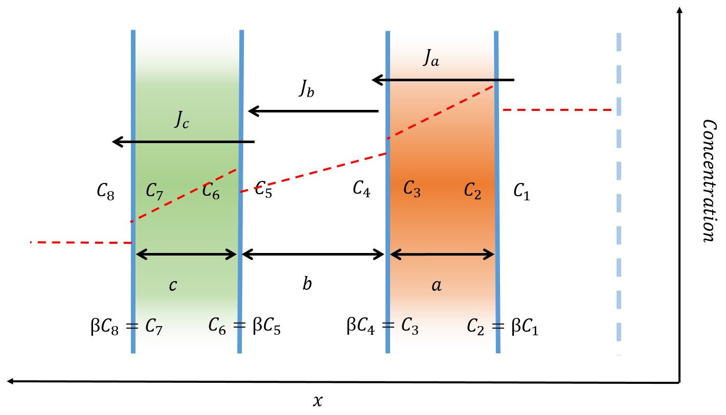
Figure 4: The diffusion of a small molecule across a double semi-permeable membrane. The red line indicates the concentration level before equilibrium is reached. The small molecule is more soluble within the membrane resulting in a higher concentration just within the membrane.

The volume of the periplasm and inner cell must be known in order to calculate the concentration of $C_4$, $C_5$ and $C_8$. The diffusivity of TNT in the membrane ($D_m$) will be less than the diffusivity in water due to the presence of the lipids. Therefore setting $D_m = D_w$ will give us the maximum rate of diffusion across the membrane.

A value for the partition coefficient was investigated in in vivo Activity

A Spatial Model

To introduce the concept of position into our model, we created a naive simulation of the growth of the bacterial population. Importantly, in this program, each individual bacterium was modelled separately. The bacterium had a position on a grid and each was modelled over a certain period of time.

In addition, the program also simulated a kill switch, which worked by producing holin when there was no TNT in the cell, and then killing the cell if it reached a certain amount. Such kill switches are common in the Registry (e.g. Part:BBa_K302035). In order to implement such a kill switch it would be necessary for the cells to sense the concentration of TNT and, in order to simulate various outcomes, the response to TNT would need to be characterised. We therefore identified and characterised key promoter elements that can respond to TNT and/or nitroglycerin (see Detection of Xenobiotics).

Each cell in the grid has an amount of TNT present and is either empty or occupied by a bacterium. At each time interval, if there was a bacterium in the cell, an amount of TNT proportional to the difference between the amount outside the bacterium and the amount inside the bacterium would diffuse across the membrane, i.e.:

\begin{equation} R=k(\text{TNT}_{\text{out}}−\text{TNT}_{\text{in}}) \end{equation}

where ‘$R$’ is the rate of diffusion and ‘$k$’ is an arbitrary constant.

The bacteria would each have an amount of TNT and an amount of holin associated with them. At each time interval, they had a chance to split into two bacteria, and if so the concentrations of the substances would be divided equally. The bacterium would only split if there was at least one empty space in the eight cells surrounding it, and the chance that it would split is proportional to the number that were free.

They would also die if the holin level reached a certain threshold or the TNT level reached a certain threshold. This will model the fact that TNT could be toxic to the bacteria. For more information see E. coli's Xenobiotic Tolerance.

At each interval, the amount of TNT in the bacterium would be reduced by a random amount which was proportional to the amount currently in the bacterium. In the visualisation of this model, the colour of each grid cell and each bacterium was represented by the amount of TNT in it. The variation in colour is proportional to the logarithm of the amount of TNT so that the exponential decrease can be seen more clearly. Finally, the volume of the music accompanying the simulation is proportional to the number of cells in the population.

These different examples of our model show the effectivness of the kill switch. We wanted to ensure that the bacteria would not continue to grow in an area where there was no TNT. However, we also needed the bacteria to have some ability to spread across such regions. For a particular set of values, we were able to find how far, on average, the bacteria would spread. Here, the model has been run three times with different distributions of TNT.

Figure 5: The areas of TNT are far apart. The bacteria is unable to spread between regions.

Figure 6: The areas of TNT are closer together. The bacteria managed to reach the second region.

Figure 7: The areas of TNT are close together. The bacteria can easily propogate over the whole region.

It is clear from these figures that the bacteria can only spread a certain distance. The model was based on a set of parameters that were unknown to us, but by tuning the growth rate of the bacteria and the production rate of XenB, we could change the maximum distance.

Summary

The main conclusions that we can draw from the model regarded the design of the kill switch. We discovered that we need to make sure that the growth rate of the bacteria may affect it such that it spreads further than we wanted, and that with a threshold kill switch we would need to make sure that the bacteria would eventually die. This would depend on the different constants.

However, we found that it was difficult to find all the values of the different constants, even with only a simple mathematical model. Creating a visual model mitigated this somewhat as it allowed us to easily see what would happen in different situations. Regardless, our discoveries informed our choice of experiments in the next section of the project.

The models also influenced our choice of experiments. This was done by identifying constants that would need to be quantified and designing experiments around them. The constants and their corresponding experiments are listed below:

Coefficient	Experiment
$g$, $d$	The Toxicity of TNT and Nitroglycerin to E. coli.
$V_{\text{max}}$, $k_m$	Validation of Enzyme Function and Activity
$m$	in vivo Activity

References

ALKALINE HYDROLYSIS OF TNT, Yi-Ching Wu, 2001

Navigation

Previous: Our Project

Next: The Enzymes