Stochastic Model.

Until now, all we have is a deterministic model of our system of detection of Cholerae. This model takes into account exact concentrations of molecules as the variables in the differential equations. This means that we make calculations with the mean values of the amount of molecules. It is well known that we can simulate this kind of molecular dynamics as stochastic processes. In particular, such events will be simulated as Markovian random walk in N dimension, where N represents the number of substances involved.

“…For “ordinary” chemical systems in which fluctuations and correlations play no significant role, the method stands as an alternative to the traditional procedure of numerically solving the deterministic reaction rate equations. For nonlinear systems near chemical instabilities, where fluctuations and correlations may invalidate the deterministic equations, the method constitutes an efficient way of numerically examining the predictions of the stochastic master equation. Although fully equivalent to the spatially homogeneous master equation, the numerical…” (Gillespie 1976)

Dealing with such a processes, the first possible approach will be to solve the stochastic master equation. The function that satisfies that equation will measure the probability of finding different numbers of molecules of the N different substances at each instant of time. But as you should probably know, this kind of numerical computation will be hard to develop and won’t be efficient. One of the reason is, for example, that, due to the very low probability of occurrence of the events (chemical reactions, ARN transcription, proteins production, …), and the very short time intervals that we should use, most of the time won’t be happening nothing.

For that reason, we decided to use a nice very efficient algorithm proposed by Daniel Gillespie, which is based in a different probability function density: The reaction probability density function. These functions will tell us how much time will pass until the next event occurrence and how this time is distributed. After that we decided which one of the events will occur based on the number of molecules of each species and how they interact with each other.

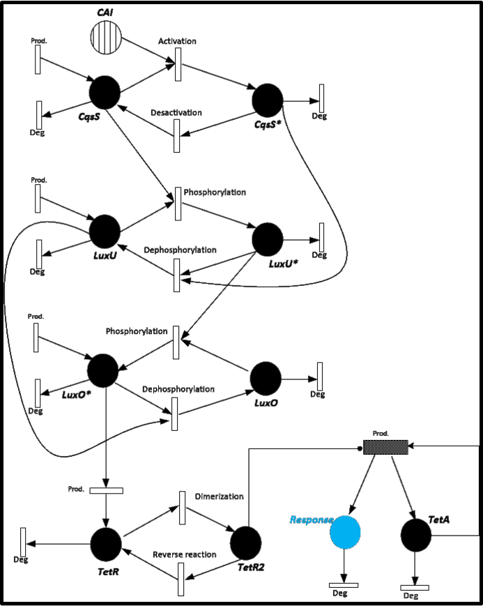
To give you an idea of how does our system works and how will be the events related, we present a Stochastic Petri Net. In Figure 1 we can appreciate the different molecules species interacting between them or undergoing process such as degradation or production.
<

Figure 1
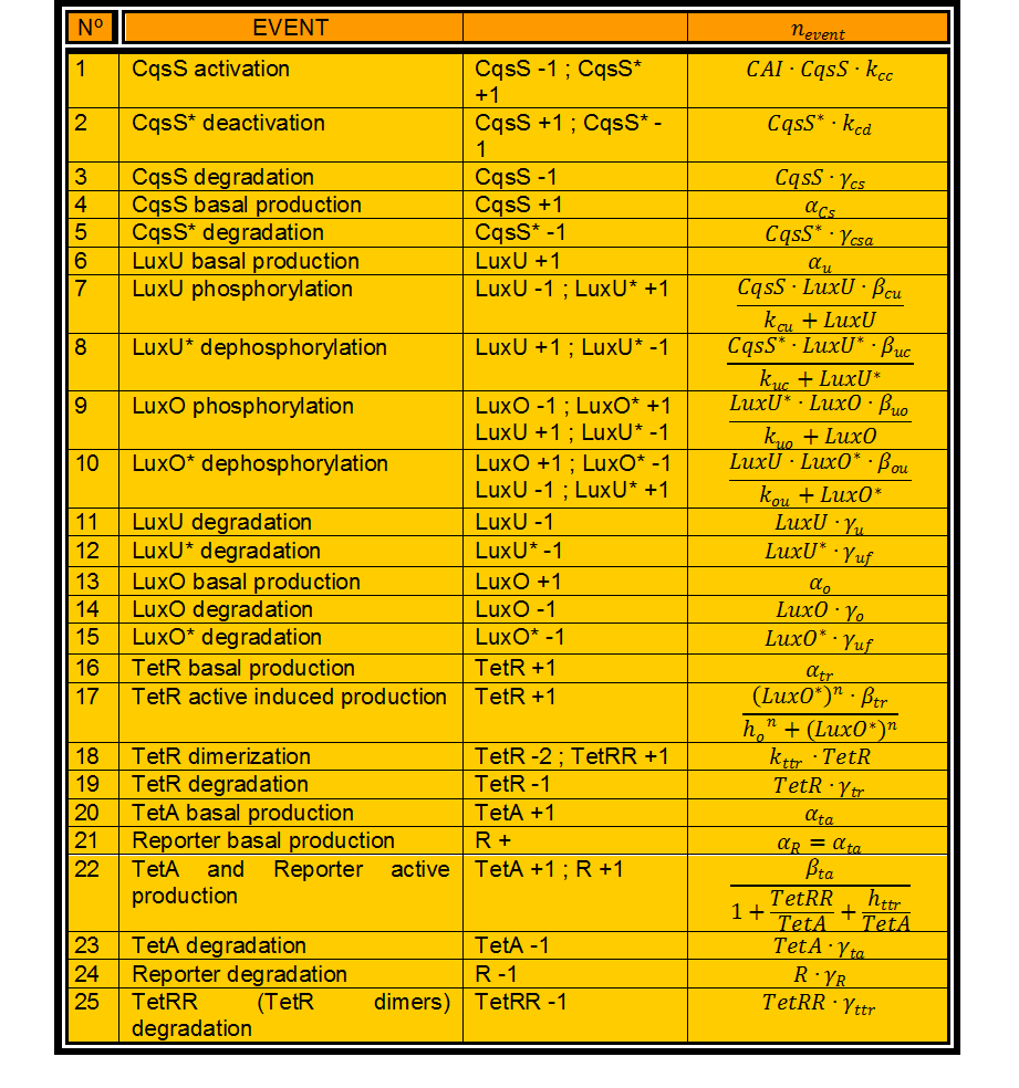
In this case, we have 24 different possible events to take into account. (Table 1)

Table 1. Events involved in our detection system. In Table 1 every variable represents the number of molecules of this kind. n_events is then a real number.



The time τ between events is calculated by:

Which event will occur is calculated by using another random number R between 0 and 1 in the following way:

Let’s define

Now divide [0,1] in 25 interval such that (Figure 2)

Figure 2

The size of the ith interval depends on the value of n_i.
The event that will occur is the one that correspond to in which interval is located the random number R.

Results

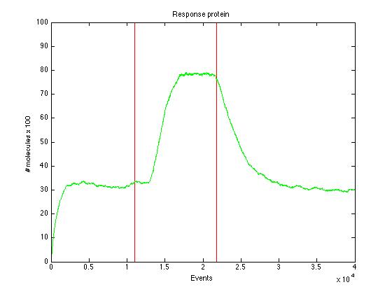
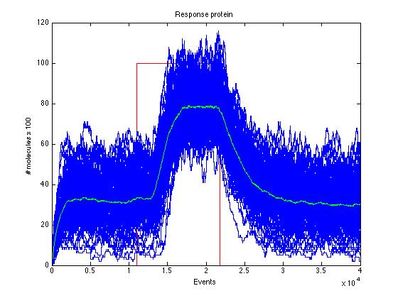
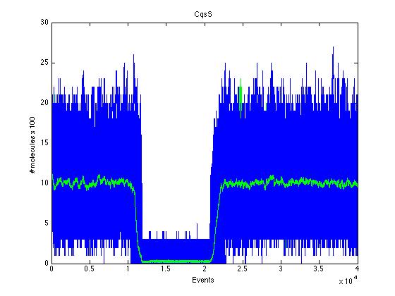
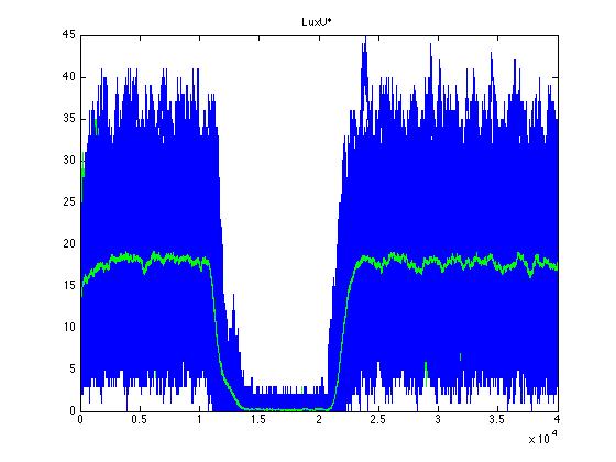
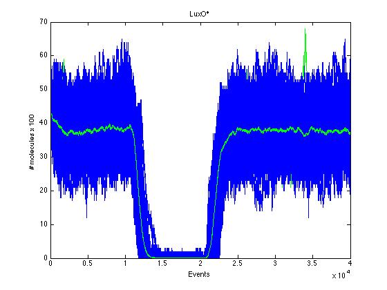
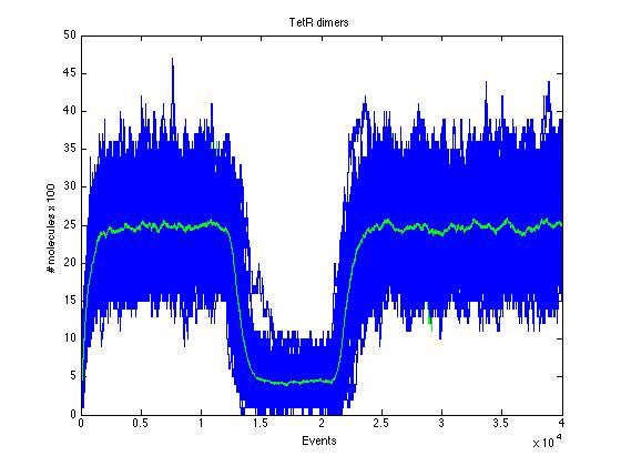
Here we present a graphic for each molecule species involved in our system and how it responds to the presence of CAI-1 in the environment. The red line in the Figure 3 represents the amount of CAI-1 molecules in the environment.
The blue lines represent the behavior of each cell and the green line presents the mean behavior of the total population.
As we can see CqsS and CqsS* have oposing (complementary) behaviors as we would expect this can be seen in figures 5 and 6 Same goes for LuxU and LuxU*, and LuxO and LuxO* in figures 7, 8, 9 and 10 respectively
Also in figure 11 can be seen how such a small change in TR has a drastic effect in the TR dimer.

Figure 3

Figure 4

Figure 5

Figure 6

Figure 7

Figure 8

Back to modeling

Go!