Team:Paris Saclay/Modeling/bacterial Growth
From 2014.igem.org
m (→References) |
m (→General conclusion : What about lemon ?) |
||
| Line 319: | Line 319: | ||
In practise, we use genetically modified ''E.coli''. As the modification that we carried out do not touch to the vital metabolism of bacteria we may assume that the originel ''E.coli'''s birth and death rate have not been changed. | In practise, we use genetically modified ''E.coli''. As the modification that we carried out do not touch to the vital metabolism of bacteria we may assume that the originel ''E.coli'''s birth and death rate have not been changed. | ||
| - | So, according to the research of | + | So, according to the research of Eric Stewart [https://2014.igem.org/Team:Paris_Saclay/Modeling/bacterial_Growth#References [Ste]], we have |
\[ \lambda = 3,6 \times 10^{-2} ~ min^{-1} \] | \[ \lambda = 3,6 \times 10^{-2} ~ min^{-1} \] | ||
and | and | ||
Revision as of 22:43, 16 October 2014

Contents |
Bacterial Population Growth
We are here considering a bacterial population uniformly spread on a surface in the euclidian space, in crowd-free conditions and with unlimited food resource.
In order to be as instructive as possible, we will process in two time : first we will consider that bacteria never die, then - and because the previous assumption is obviously no realistic - we will consider that bacteria can breed and die.
Each time, we will expose a deterministic and a stochastic model. The major advantage of the deterministic one is his simplicity. But this simplicity has a cost : while every set of variable states is uniquely determined by parameters in the model and by sets of previous states of these variables, the deterministic models perform the same way for a given set of initial conditions which is not really desirable. Conversely, in a stochastic model, randomness is present, and variable states are not described by unique values, but rather by probability distributions.
Menu
Pure birth process
In this part, we assume that :
- bacteria do not die,
- they develop without interacting with each other,
- the birth rate, $\lambda$, is the same for all the organisms, regardless of their age and does not change with time.
Determininistic model
Let $N(t)$ denote the population size at time $t$.
Then in the subsequent small time interval of length $h$ the increase in the population due to a single organism is $\lambda\times h$ - i.e the rate $\times$ the time - so the increase in size due to all $N(t)$ organisms is $\lambda\times h\times N(t)$. Thus \[ N(t+h) = N(t) + \lambda h N(t) +o(h) \] which on dividing both sides by h gives \[ \frac{N(t+h)-N(t)}{h} = \lambda N(t)+o(1) \] Letting $h$ approach zero then yields the differential equation \[ \frac{dN}{dt}(t) = \lambda N(t) \] which integrates to give \[ N(t) = N_0 e^{\lambda t} \] where $N_0$ denotes the initial population size at time $t=0$. This form for $N(t)$ is known as the Malthusian expression for population development, and shows that the simple rules we used rises to exponential growth.
Stochastic model
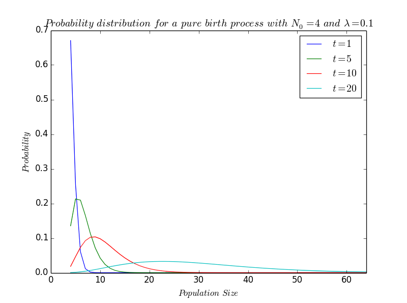
A deterministic model only give us an average solution of the problem. In order to take into account the unpredictability of biology, we need a stochastic approach. Usualy, the stochastic model converge to a limit which is similar to the deterministic model. A stochastic model is all the more pertinent as the initial bacterial population is small. It give us an array of probabilities, describing each possible state for the population at time t.
As in the deterministic model, we call $\lambda$ the birth rate : in a short time interval of length $h$ the probability that any particular cell will divide is $\lambda h$. Then for the population to be of the size $N$ at the time $t+h$, either it is of the size $n$ at time $t$ and no birth occurs in the subsequent short interval $(t,t+h)$, or else it is of size $N-1$ at time $t$ and exactly one birth occurs in $(t,t+h)$. In fact, by choosing $h$ sufficiently small we may ensure that the probability of more than one birth occuring is negligible.
Since the probability of $N$ increasing to $N+1$ in $(t,t+h)$ is $\lambda h N$, it follows that the probability of no increase in $(t,t+h)$ is $1-\lambda h N$. Similarly, the probability of $N-1$ increasing to $N$ in $(t,t+h)$ is $\lambda(N-1)h$. Thus on denoting \[ p_N(t)(t) = \mathbb{P}(population~is~of~size~N~at~time~t) \] we have \[ p_N(t+h) = p_N(t)\times\mathbb{P}(no~birth~in~(t,t+h)) + p_{N-1}(t)\times\mathbb{P}(one~birth~in~(t,t+h))+o(h) \] i.e \[ p_N(t+h) = p_N(t)\times(1-\lambda N h)+p_{N-1}(t)\times\lambda(N-1)h+o(h) \] On dividing both sides by $h$ \[ \frac{p_N(t+h)-p_N(t)}{h} = - \lambda N p_N(t)+\lambda(N-1)p_{N-1}(t)+o(1) \] and as it approaches zero this becomes \[ \frac{dp_N}{dt}(t) = \lambda(N-1)p_{N-1}(t)-\lambda p_N(t) \] for $N=N_0,~N_0+1,...$.
The solution of the above give equation is \[ p_N(t) = \left( \begin{array}{c} N-1 \\ N_0-1 \end{array} \right) e^{-\lambda N_0 t}(1-e^{-\lambda t})^{N-N_0} \quad;\quad N=N_0, N_0+1,... \] which is the negative binomial distribution where, for conveniance, we have written $N(0)$ as $N_0$. In a pratical way, this differential equation can be solved by a variety of theoretical techniques. While we are more interested here with the result than the mathematical formulae, we let the readers interested in the proof consult Bailey's book The elements of stochastic processes [Bai], for instance.
As our solution is of standard negative binomial form, the mean -i.e the average value- and the variance -i.e the average way we move away from the mean- are given by : \[ m(t)=N_0e^{\lambda t}\quad and\quad V(t)=N_0e^{\lambda t}(e^{\lambda t}-1) \]
Especially, we see that the mean of the stochastic model is exactly what we have found by having a deterministic approach.
Simple birth-death process
In fact, the model we exposed in the previous part was not realistic and we have to consider that our bacteria could also die. We introduce here the death rate $\mu$ which is also supposed be the same for all bacteria, regardless of their age and don't change with time, and we still asume that bacteria develop whihout interacting with each other.
Determininistic model
We still have the same notation and $N(t)$ denote the population size at time $t$.
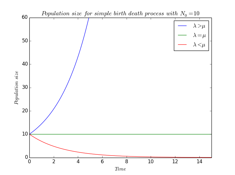
We proceed in a same way than in the pure birth process but, this time, death will lead to a decrease of the population, that's why the $\mu$ is preceded by a minus : \[ \frac{dN}{dt}(t) = (\lambda-\mu) N(t) \] which integrates to give \[ N(t) = N_0 e^{(\lambda-\mu) t} \] where $N_0$ denotes the initial population size at time $t=0$.
We still find an exponential growth, but the coefficient $(\lambda-\mu)$ can now be either positive or either negative in function of the values of $\lambda$ and $\mu$.
Stochastic model
Establishment of the model
Analysis of the stochastic behaviour follows along exactly the same lines as for the pure birth process, except that in the sort time $(t,t+h)$, there is now a probability $\lambda h$ that a particular bacterium gives birth \emph{and} a probability $\mu h$ that it dies. With a population of size $N(t)$ at sime $t$, the probability that no events ocures is therefore $1-\lambda Nh-\mu Nh$, since $h$ is assumed to be sufficiently smal to ensure that the probability of more than one event occuring in $(t,t+h)$ is negligible.
As state $N$ can be reached from states $N-1$ (by a birth), $N+1$ (by a death) or $N$ (either), we find : \[ p_N(t+h) = p_N(t)\times(1-(\lambda+\mu)N h)+p_{N-1}(t)\times\lambda(N-1)h+p_{N+1}(t)\times\mu(N+1)h+o(h) \] Dividing by $h$ and letting $h$ approach zero then yields the set of equations \[ \left\{ \begin{array}{l} {\displaystyle \frac{dp_N}{dt}(t) = \lambda(N-1)p_{N-1}(t)-(\lambda+\mu)N p_N(t)+\mu(N+1)p_{N+1}(t)} \\ {\displaystyle p_N(0)=\delta_{N,N_0}} \end{array}\right. \] over $N=0,1,2\ldots$ and $t\geqslant0$ on which, for $N=0$, $p_{-1}(t)$ is identically zero.
Generating function $\star$
For the following part, the reader could refer to the book of Cox and Miller, The Theory of Stochastic Processes [Mil]. Let \[ \forall(z,t)\in\mathbb{R}^+*\times\mathbb{R}^+*,\quad G(z,t) = \sum_{n=0}^{\infty}p_n(t)z^n \] thus, $P_N(t)$ will be the coefficient before $z^N$ on $G(z,t)$. While $\forall t\in\mathbb{R}^+$, $p_N(t)\in[0,1]$ and we just consider the case of restricting $z$ to $\mathbb{R}^+*$ $G$ as a sence in $\overline{\mathbb{R}^+}~=~\mathbb{R}^+\cup\{+\infty\}$. We multiply the previous equation by $(z^0,z^1,z^2,\ldots)$ and add to obtain : \[ \begin{array}{rcl} {\displaystyle \sum_{n=0}^{\infty} \frac{dp_n}{dt}(t) z^n} &=& {\displaystyle \sum_{n=0}^{\infty} (\lambda(n-1)p_{n-1}(t)-(\lambda+\mu)p_n(t)+\mu(n+1)p_{n+1}(t))z^n} \\ &=& {\displaystyle \lambda \sum_{n=0}^{\infty}p_{n-1}(t)(n-1)z^n - (\lambda+\mu)\sum_{n=0}^{\infty}p_n(t)nz^n + \mu\sum_{n=0}^{\infty}p_{n+1}(n+1)z^n} \end{array} \] and while we know that $p_{-1}=0$ \[ \begin{array}{rcl} {\displaystyle \sum_{n=0}^{\infty} \frac{dp_n}{dt}(t) z^n} &=& {\displaystyle \lambda \sum_{n=0}^{\infty}p_{n}(t)(n)z^{n+1} - (\lambda+\mu)\sum_{n=0}^{\infty}p_n(t)nz^n + \mu\sum_{n=0}^{\infty}p_{n}(n)z^{n-1}} \\ &=& {\displaystyle \lambda z^2\sum_{n=0}^{\infty}p_{n}(t)(n)z^{n-1} - (\lambda+\mu)z\sum_{n=0}^{\infty}p_n(t)nz^{n-1} + \mu\sum_{n=0}^{\infty}p_{n}(n)z^{n-1}} \\ &=& {\displaystyle (\lambda z^2-(\lambda+\mu)z+\mu) \sum_{n=0}^{\infty}p_{n}(t)(z^n)'} \end{array} \] and finally \[ {\displaystyle \frac{\partial G}{\partial t}}(z,t) ~=~{\displaystyle (\lambda z^2-(\lambda+\mu)z+\mu)\frac{\partial G}{\partial z}(z,t)} ~=~{\displaystyle (\lambda z-\mu)(z-1)\frac{\partial G}{\partial z}(z,t)} \] which can be written as \[ \partial_tG(z,t)+f(z)\partial_zG(z,t) = 0\quad where\quad f(z) := -(\lambda z-\mu)(z-1) \]
Lax-Milgram theorem $\star\star$
We will try to apply the Lax-Milgram theorem in the following paragraph. Readers which are not familiar with the theory of distribution and how to use it in order to solve partial derivative equation (PDE) could consult the notes of N.Burq and P.Gerard Contrôle optimal des équations aux dérivees partielles [Bur].
As from now, we work in the space of distributions, $\mathcal{D}(\mathbb{R^2})$. Morever, we assume that the reader knows that $\mathbb{R}^+*\times\mathbb{R}^+*~\approx~\mathbb{R}^2$ -$\exp$ defines a bijection between $\mathbb{R}$ and $\mathbb{R}^+*$- and we will juste write $\mathbb{R}^2$ instead of $(\mathbb{R}^+*)^2)$. To all agree with the notation, we remind (or not) the definition of a Sobolev space. First we define \[ \mathcal{H}^1(\mathbb{R^2})=\{\phi\in\mathbb{L}_2(\mathbb{R^2})~|~\triangledown\phi\in\mathbb{L}_2(\mathbb{R}^2)\} \] In particular, we have \[ \mathcal{H}^1(\mathbb{R^2})\subset\mathcal{C}^{\infty}_0=\{\phi\in\mathcal{C}^\infty(\mathbb{R}^2)~|~Supp(\phi)~is~compact\} \] thus justify to set down \[ \mathcal{H}^1_0(\mathbb{R^2}) = \overline{\mathcal{C}^{\infty}_0(\mathbb{R}^2)}^{\mathcal{H}^1(\mathbb{R}^2)}\subseteq\mathcal{H}^1(\mathbb{R}^2) \] where $\overline{\ldots}^{\mathcal{H}^1}$ is a notation to say adherance in $\mathcal{H}^1$. $\mathcal{H}^1_0$ is an exemple of a Sobolev space. So, like the whole Sobolev space, it is an Hilbert space and we note $<~|~>$ his scalar product. \[ \forall u,v\in\mathcal{H}^1_0,\quad < u~|~v>~=~< u~|~v>_{\mathcal{H}^1_0}~:=~< u~|~v>_{\mathbb{L}^2}+< \triangledown u~|~\triangledown v>_{\mathbb{L}^2} \]
\[ \begin{array}{l} {\displaystyle \forall(z,t)\in\mathbb{R}^2,\quad\partial_tG(z,t)+f(z)\partial_zG(z,t) = 0\quad} \\ {\displaystyle \quad\quad\Leftrightarrow\quad\forall\phi\in\mathcal{C}^{\infty}_0(\mathbb{R}^2),\quad< \partial_tG+f\partial_zG~|~\phi> =0} \\ {\displaystyle \quad\quad\Leftrightarrow\quad\forall\phi\in\mathcal{C}^{\infty}_0(\mathbb{R}^2),\quad \int{\partial_tG\phi+f\partial_zG\phi} = 0} \\ {\displaystyle \quad\quad\Leftrightarrow\quad\forall\phi\in\mathcal{C}^{\infty}_0(\mathbb{R}^2),\quad a(G,\phi) = 0\quad where\quad a(G,\phi)=\int{\partial_tG\phi+f\partial_zG\phi}} \end{array} \]
Because of the linearity of the integral, $a$ is a bilinear form. So we just have to proof that $a$ is continue and coercive.
- $a$ is continue :
\[ \begin{array}{rcl} {\displaystyle |~a(u,\phi_n)~|=|~\int_{\mathbb{R}^2}{\partial_tu\phi_n+f\partial_zu\phi_n}~|} &=& {\displaystyle |~\int_{Supp(\phi_n)}{\partial_tu\phi_n+f\partial_zu\phi_n}~|} \\ &\leqslant& {\displaystyle \int_{Supp(\phi_n)}{|~\partial_tu\phi_n+f\partial_zu\phi_n~|}} \\ &\leqslant& {\displaystyle \int_{Supp(\phi_n)}{|~\phi_n~|.|~\partial_tu+f\partial_zu~|}} \end{array} \] The Cauchy-Schwar's inequality give us \[ \begin{array}{rcl} |~a(u,\phi_n)~|&\leqslant&\sqrt{ {\displaystyle\int_{Supp(\phi_n)}{|~\phi_n~|^2}}}\times\sqrt{{\displaystyle\int_{Supp(\phi_n)}{|~\partial_tu+f\partial_zu~|^2}}} \\ &\leqslant& ||\phi_n||_{\mathbb{L}_2}\times\sqrt{{\displaystyle\int_{Supp(\phi_n)}{|~\partial_tu+f\partial_zu~|^2}}} \end{array} \] Well, \[ \begin{array}{crl} |~\partial_tu+f\partial_zu~|&\leqslant&\max(1,\underset{x\in Supp(\phi_n)}\sup f(x)) |~\partial_tu+\partial_zu~| \\ |~\partial_tu+f\partial_zu~|^2&\leqslant&[\max(1,\underset{x\in Supp(\phi_n)}\sup f(x))]^2 |~\partial_tu+\partial_zu~|^2 \\ \int_{Supp(\phi_n)}{|~\partial_tu+f\partial_zu~|^2}&\leqslant&[\max(1,\underset{x\in Supp(\phi_n)}\sup f(x))]^2\int_{Supp(\phi_n)}{ |~\partial_tu+\partial_zu~|^2} \\ \sqrt{{\displaystyle\int_{Supp(\phi_n)}{|~\partial_tu+f\partial_zu~|^2}}}&\leqslant&[\max(1,\underset{x\in Supp(\phi_n)}\sup f(x))]\sqrt{{\displaystyle\int_{Supp(\phi_n)}{ |~\partial_tu+\partial_zu~|^2}}} \\ \sqrt{{\displaystyle\int_{Supp(\phi_n)}{|~\partial_tu+f\partial_zu~|^2}}}&\leqslant&[\max(1,\underset{x\in Supp(\phi_n)}\sup f(x))].||u||_{\mathbb{L}_2} \end{array} \] So \[ {\displaystyle |~a(u,\phi_n)~|\leqslant||\phi_n||_{\mathbb{L}_2}\times[\max(1,\underset{x\in Supp(\phi_n)}\sup f(x))].||u||_{\mathbb{L}_2}} \]
Let ${\displaystyle M=\underset{n\in\mathbb{N}}{\sup}\max(1,\underset{x\in Supp(\phi_n)}\sup f(x))}$. And the Heine theorem assure that $M$ is finit. Actually, $f$ is continue on the compact $Supp(\phi_n)$ for all $n$ in $\mathbb{N}$ so is bound on it. By passing to the limit, we find \[ {\displaystyle |~a(u,v)~|\leqslant (1+M)||u||_{\mathcal{H}^1_0}||\phi_n||_{\mathcal{H}^1_0}} \] which is what we search.
- $a$ is coercive :
With a simular calculation, we show that $a$ is coercive, i.e that it exists a constant $\alpha$ in such a way that \[ \forall u \in \mathcal{H}^1_0(\mathbb{R}^2), \quad |a(u,u)| \geqslant \alpha ||u||^2 \]
So, according to the Lax-Milgram theorem \[ \exists ! G\in\mathcal{H}^1_0,\quad\forall\phi\in\mathcal{H}^1_0,\quad a(G,\phi)=0 \] On other words, it means that, in the space of distributions, if we can exhibit a solution, it is the only solution of this problem. And the solution exists. If the solution we find is sufficiently regular (in a way to define more precisly), general theorems assure that the solution we find in not only a solution in the space of distributions but is also a solution in "the real life".
Precisely, we can verify with a computation that, if $\lambda\neq\mu$ \[ \gamma(z,t)~:=~\left(\frac{\mu(1-z)-(\mu-\lambda z)e^{-(\lambda-\mu)t}}{\lambda(1-z)-(\mu-\lambda z)e^{-(\lambda-\mu)t}}\right)^{N_0} \] is solution to the equation, i.e that \[ \forall(z,t)\in\mathbb{R}^2, \partial t\gamma(z,t)+f(z,t)\partial z\gamma(z,t)=0 \] The computation is verry long and not really interessant (it suffices to derive $\gamma$ and substitue in the equation) that's why we will not detail it in this text...
So, while the solution exists and is unique according to the Lax-Milgram theorem, if $\lambda\neq\mu$, we have found it and \[ \forall(z,t)\in\mathbb{R}^2,~G(z,t)~=~\left(\frac{\mu(1-z)-(\mu-\lambda z)e^{-(\lambda-\mu)t}}{\lambda(1-z)-(\mu-\lambda z)e^{-(\lambda-\mu)t}}\right)^{N_0} \quad(\star)\] and for all time $t$, $P_N(t)$ is the coefficient before $z^N$ in the previous expression.
Coefficient of Variation $\star\star$
In this small parts, we will just try to have an idea of the influence of the value of $\lambda$ and $\mu$ on the probability. To do that, we calcul the mean and the variance of population size. Actually, while we consider a discret probability, \[ m(t) = \sum_{n=0}^{\infty}{n p_n(t)} = \ldots = N_0 e^{(\lambda-\mu)t} \] and by a similar calcul, if $\lambda\neq\mu$, \[ V(t) = N_0\frac{\lambda+\mu}{\lambda-\mu}e^{(\lambda-\mu)t}(e^{(\lambda-\mu)t}-1) \]
Unlike $m(t)$ and $V(t)$ depend not only on the difference between the birth and the death rates, but also on their absolute magnetudes. This is what we should expect, because predictions about the future size of a population will be less precise if birth and death occur in rapid succesion than if they occur only occasionally.
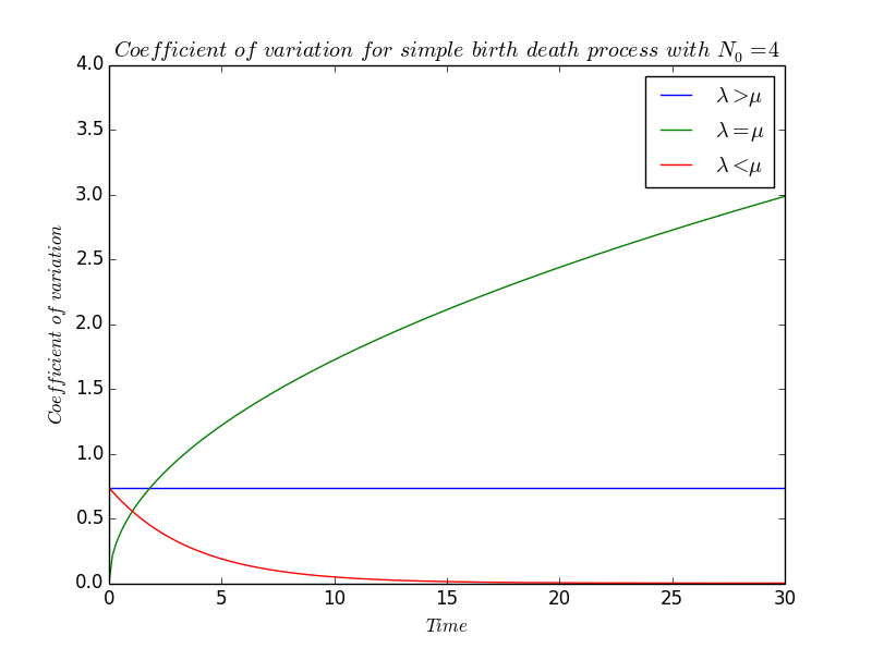
We defin the coefficient of variation $\displaystyle CV(t)~:=~\frac{\sqrt{V(t)}}{m(t)}$ which qualify the variation of the system and we will study the effect of the relative values of $\lambda$ and $\mu$. \[ \begin{array}{rcl} \forall\lambda\neq\mu,~\forall t, CV(t) &=& {\displaystyle\sqrt{N_0\frac{\lambda+\mu}{\lambda-\mu}e^{(\lambda-\mu)t}(e^{(\lambda-\mu)t}-1)}\times\frac{1}{N_0}e^{-(\lambda-\mu)t}} \\ &=& {\displaystyle \sqrt{\frac{\lambda+\mu}{N_0(\lambda-\mu)}}\times\sqrt{e^{(\lambda-\mu)t}-1}\times e^{-\frac{1}{2}(\lambda-\mu)t}} \\ &=& {\displaystyle \sqrt{\frac{\lambda+\mu}{N_0(\lambda-\mu)}}\times\sqrt{e^{(\lambda-\mu)t}-1}\times \sqrt{e^{-(\lambda-\mu)t}}} \\ &=& {\displaystyle \sqrt{\frac{\lambda+\mu}{N_0(\lambda-\mu)}}\times \sqrt{1-e^{-(\lambda-\mu)t}}} \end{array} \]
- If $\lambda\gneq\mu$,
\[ CV(t)~\sim~\sqrt{\frac{\lambda+\mu}{N_0(\lambda-\mu)}} \]
- On the contrary, if $\lambda\lneq\mu$,
\[ CV(t)~\sim~\sqrt{\frac{\lambda+\mu}{N_0(\lambda-\mu)}}\times e^{\frac{1}{2}(\lambda-\mu)t} \]
- We are now interest in the coefficient of variation when $\lambda=\mu$. We cannot find an equivalent as easily as previously while $CV$, at least in that form , is not defined for $\lambda=\mu$. Actually, to know if $CV$ is defined or not when $\lambda=\mu$ is not really interessant because we want to have an idea of what will be the behaviour of $CV$ if $\lambda$ is so much close to $\mu$ that, biologically, they seem to be equal. It will be the some idea in the folowing part.
We remind that the function $\exp:x\rightarrow e^x$ is indefinitely differentiable, i.e $\exp\in\mathcal{C}^{\infty}$ so it admits a Taylor expansion in the neighbourhood of $0$ -in particular- : $\forall n\in\mathbb{N}$ and for $t$ sufficiently near to $0$, \[ \begin{array}{rcl} e^t &=& {\displaystyle \exp(0)\frac{t^0}{0!}+\exp'(0)\frac{t^1}{1!}+\exp^{(2)}(0)\frac{t^2}{2!}+\exp^{(3)}\frac{t^3}{3!}+\ldots+\exp^{(n-1)}\frac{t^{n-1}}{(n-1)!}+\underset{t\rightarrow 0}{o}(t^n)} \\ &=& {\displaystyle 1+t+\frac{t^2}{2}+\frac{t^3}{6}+\ldots+\frac{t^{n-1}}{(n-1)!}+\underset{t\rightarrow 0}{o}(t^n)} \end{array} \] So, by devoloping the exponentional in the expression of $CV$, \[ \forall t\in\mathbb{R},~CV(t) ~=~ \sqrt{\displaystyle{\frac{\lambda+\mu}{N_0(\lambda-\mu)}}}\times\sqrt{1-(1-(\lambda-\mu)t)} +\underset{\lambda\rightarrow\mu}{o}(\sqrt{(\lambda-\mu)t})\] and cancelling the expression, we find. \[ CV(t)~=~\sqrt{{\displaystyle\frac{(\lambda+\mu)t)}{N_0}}} +\underset{\lambda\rightarrow\mu}{o}(\sqrt{t}) \] Finnaly, as $\lambda=\mu$, it comes that \[ CV(t)~\underset{\lambda\rightarrow\mu}\sim~\sqrt{{\displaystyle\frac{2\lambda t}{N_0}}} \]
At this point it is worth reflecting on a a criticism sometimes levelled against this model of exponential population growth, namely that if $\lambda$ exceeds $\mu$ then it ultimatly leads to populations so large that their existence is physically impossible.
A far more serious, but often neglected, question is How far into the future is ecological prediction, based on simple models, feasible ? The answer must depend on the situation being considered, since it is influenced to a large extent by biological factors such as over what length of time the (actual) birth and death rates can be expected to remain reasonably constant and how large $N(t)$ may become before organisms can no longer be assumed to develop independently of each other. Clearly, whenever a biological process, no matter how innocently simple it may first apprear, is being modelled, the underlying assumption used in the contruction of the model must be constantly questioned. The feasibly predictable future may well be disapointingly short.
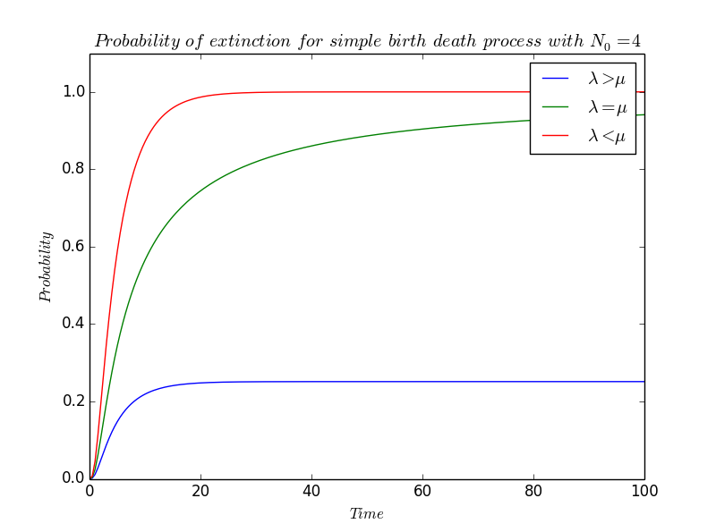
Probability of extinction $\star$
Last part but not least : we will study the probability of extinction of our bacteria population.
Intuitively, this probability will depend on $\lambda$ and $\mu$ : if $\lambda\ll\mu$, then it is reasonable to suppose that since death predominate the population will eventually \leqdie out, and since we have not consider imigration phenomen, this implies extinction. On the contrary, if $\lambda\gg\mu$ then birth predominate, and either an initial downward surge causes the population to become extinct or else $N(t)$ avoids becoming zero and the population grows indefinitely.
The probability that extinction has occured at or before $t$ is the coefficient before $z^0$ in $(\star)$, i.e, \[ \left(\frac{\mu-\mu e^{-(\lambda-\mu)t}}{\lambda-\mu e^{-(\lambda-\mu)t}}\right)^{N_0} \] where $N_0$ still refer to $N(0)$.
In particular, this value for $N_0=1$ is the probability that a single bacterium ans all his clone are extinct at or before time $t$.
To obtain the probability of ultimate extinction, $p_0(\infty)$, we have to let $t$ tend ti infinity and
- If $\lambda\gneq\mu$,
\[ p_0(\infty)~\sim~\left(\frac{-\mu e^{\mu t}}{-\mu e^{\mu t}}\right)^{N_0}~=~1~\longrightarrow 1 \] Ultimate extinction is therefore certain.
- On the contrary, if $\lambda\lneq\mu$, then the exponential terms vanish, so
\[ p_0(\infty)~\sim~\left(\frac{\mu}{\lambda}\right)^{N_0}\longrightarrow\left(\frac{\mu}{\lambda}\right)^{N_0} \] In particular, even though $\lambda$ is greater than $\mu$, extinction can still occure. It must append when $N_0$ is small os when $\displaystyle \frac{\mu}{\lambda}$ is near one.
Thus, if we wish to choose $N_0$ to ensure that $p_0(\infty)\leqslant 10^{-3}$, then we require \[ \left(\frac{\lambda}{\mu}\right)^{N_0}\geqslant 10^3 \] i.e \[ log_{10}\left(\left(\frac{\lambda}{\mu}\right)^{N_0}\right)~=~N_0 log_{10}\left(\frac{\lambda}{\mu}\right)\geqslant 3 \] and finnaly, \[ N_0\geqslant\frac{3}{\left(\frac{\lambda}{\mu}\right)^{N_0}} \]
For example, if $\mu=1$ and \[ \lambda=1.01,\quad 2,\quad 10,\quad 100,\quad 1000, \] $No$ must be choosen such as \[ N_0\geqslant 695,\quad 73,\quad 10,\quad 3,\quad 2,\quad 1. \]
- It is a little bit more difficult to determine $p_0(\infty)$ when $\lambda=\mu$ because the expression $(\star\star)$ is not defined when $\lambda=\mu$. But, by reminding that the exponentional is $\mathcal{C}^\infty$ on $\mathbb{R}$ -so particuliary on $0$- and admit so a Taylor-expansion in the neighborhood of $0$ :
\[ e^t~=~1+t+\frac{t^2}{2}+\frac{t^3}{6}+\frac{t^4}{24}+\ldots+\underset{t\rightarrow 0}{o}(t^n) \] we can write $p_0$ as \[ p_0(t) = \left(\frac{{\displaystyle\mu-\mu(1-(\lambda-\mu)t+\underset{\lambda\rightarrow\mu}{o}((\lambda-\mu)t)}}{{\displaystyle\lambda-\mu(1-(\lambda-\mu)t+\underset{\lambda\rightarrow\mu}{o}((\lambda-\mu)t)}}\right)^{N_0} = \left(\frac{{\displaystyle \mu(\lambda-\mu)t+\mu\underset{\lambda\rightarrow\mu}{o}((\lambda-\mu)t)}}{{\displaystyle\lambda-\mu+\mu(\lambda-\mu)t+\mu\underset{\lambda\rightarrow\mu}{o}((\lambda-\mu)t)}}\right)^{N_0} \] This expression simplifies, by dividing by $\lambda-\mu$, to give \[ p_0(t) = \left(\frac{{\displaystyle \mu t+\underset{\lambda\rightarrow\mu}{o}(\mu t)}}{{\displaystyle 1+\mu t+\underset{\lambda\rightarrow\mu}{o}(\mu t)}}\right)^{N_0} \underset{\lambda\rightarrow\mu}{\sim}{\displaystyle\left(\frac{\mu t}{1+\mu t}\right)^{N_0}} \] As $t$ increases, \[ p_0(t)~\underset{\begin{array}{c}{\scriptstyle \lambda\rightarrow\mu} \\ {\scriptstyle t\rightarrow\infty}\end{array}}\sim~\left(\frac{\mu t}{\mu t}\right)^{N_0}~\underset{\begin{array}{c}{\scriptstyle \lambda\rightarrow\mu} \\ {\scriptstyle t\rightarrow\infty}\end{array}}\longrightarrow~1 \] and so ultimate extinction is certain even tough the birth and the death rate are equal.
General conclusion : What about lemon ?
To come back to our lemon, let see what append when we now consider "our" bacteria and not only a general bacterium species !
In practise, we use genetically modified E.coli. As the modification that we carried out do not touch to the vital metabolism of bacteria we may assume that the originel E.coli's birth and death rate have not been changed.
So, according to the research of Eric Stewart [Ste], we have \[ \lambda = 3,6 \times 10^{-2} ~ min^{-1} \] and \[ \mu = 4,6 \times 10^{-4} min^{-1} \]
References
[Bai] Norman T.J Bailey, The Elements of Stochastic Processes with Applications to the Natural Sciences, New York, Wiley (1964).
[Bur] Nicolas Burq & Patrick Gérard, Contrôle optimal des équations aux dérivées partielles, Ecole polytechnique (2002)
[Mil] D.R. Cox & H.D. Miller, The Theory of Stochastic Processes, London : Methuen (1965)
[Ren] Eric Renshaw, Modelling Biological Populations in Space and Times, Cambridge university press (1991).
[Ste] Eric J. Stewart, Aging and Death in an Organism That Reproduces by Morphologically Symmetric Division on [http://www.plosbiology.org/article/info%3Adoi%2F10.1371%2Fjournal.pbio.0030045 PLOS Biology]
 "
"


