Team:Paris Saclay/Modeling/odor
From 2014.igem.org
(→Basic model) |
(→Results) |
||
| (2 intermediate revisions not shown) | |||
| Line 1: | Line 1: | ||
{{Team:Paris_Saclay/modeling_header}} | {{Team:Paris_Saclay/modeling_header}} | ||
| - | = | + | = Testing the Lemon scent= |
To synthesize the smell of lemon, we have to mainly produce Limonene, Geraniol and Pinene. The combination of these products will allow us to get the fragrance we need. We propose here a study of the evolution of these concentrations over time by using the technique Michaelis-Menten proposed in 1913 by Leonor Michaelis and Maud Menten. This will allow us to obtain a description of the kinetics of reactions between an enzyme (biological catalyst) and a substrate for giving a product. | To synthesize the smell of lemon, we have to mainly produce Limonene, Geraniol and Pinene. The combination of these products will allow us to get the fragrance we need. We propose here a study of the evolution of these concentrations over time by using the technique Michaelis-Menten proposed in 1913 by Leonor Michaelis and Maud Menten. This will allow us to obtain a description of the kinetics of reactions between an enzyme (biological catalyst) and a substrate for giving a product. | ||
| Line 49: | Line 49: | ||
| - | * the concentration of substrate is very large relative to the concentration of enzyme: $[S] >> [E]_T $ and the concentration of the product is negligible: $P \approx 0$. With the equation $ES | + | * the concentration of substrate is very large relative to the concentration of enzyme: $[S] >> [E]_T $ and the concentration of the product is negligible: $P \approx 0$. With the equation $ES \underset{k_{-2}}{\longleftarrow} E + P$, we know that the speed formation of $ES$ is gived by $v = k_{-2}[E][P] \approx 0$. |
* We suppose that we reach the equilibrium between $[E], [S]$ and $[ES]$ fastly. In the case of equilibrium, $[ES]$ is constant until $[P] \approx 0$, and so $\frac{d[ES]}{dt} = 0$. | * We suppose that we reach the equilibrium between $[E], [S]$ and $[ES]$ fastly. In the case of equilibrium, $[ES]$ is constant until $[P] \approx 0$, and so $\frac{d[ES]}{dt} = 0$. | ||
| Line 151: | Line 151: | ||
However, the production rates of limonene, geraniol and pinene are differents. By placing the evolutions of their concentrations in the same figure and for differents time sequences, we observe a kind of convergence of the three concentrations. | However, the production rates of limonene, geraniol and pinene are differents. By placing the evolutions of their concentrations in the same figure and for differents time sequences, we observe a kind of convergence of the three concentrations. | ||
| - | This means that after a while, limonene, geraniol and pinene have the same concentrations: a balance will thus settle. This phenomenon is represented by the images below. | + | This means that after a while, limonene, geraniol and pinene have the same concentrations: a balance will thus settle. This phenomenon is represented by the images below where concentration are in µM (micromolar) and times in minute. |
Latest revision as of 00:25, 18 October 2014

Contents |
Testing the Lemon scent
To synthesize the smell of lemon, we have to mainly produce Limonene, Geraniol and Pinene. The combination of these products will allow us to get the fragrance we need. We propose here a study of the evolution of these concentrations over time by using the technique Michaelis-Menten proposed in 1913 by Leonor Michaelis and Maud Menten. This will allow us to obtain a description of the kinetics of reactions between an enzyme (biological catalyst) and a substrate for giving a product.
Basic model
At first reading, you can skip this part and assume given the Michaelis-Menten equation.
We consider the reations below between the enzyme $E$ and the substrate $S$. $ES$ is an complex foregoing the formation of the product P.
\[ E + S \overset{k_1}{\longrightarrow} ES \overset{k_2}{\longrightarrow} E + P \]
\[ E + S \underset{k_{-1}}{\longleftarrow} ES \underset{k_{-2}}{\longleftarrow} E + P \]
where
\[ \left\lbrace \begin{array}{llll} k_1 \text{ is the association constant of } E \text{ and } S \\ k_{-1} \text{ is the dissociation constant of } ES \\ k_2 \text{ is the reaction constant of } ES \text{ in } E + P \\ k_{-2}\text{ is the association constant of } E \text{ and } P \\ \end{array} \right. \]
We want to model the kinetics of the reaction catalyzed by enzymes Michaelis. We are interested in the concentration of molecules and various constants that we have described above.
The speed of the reaction $V$ is caracterised by the speed of apparition of the product. It is given by $V = \frac{d[P]}{dt}$ where $[P]$ is the concentration of the product. Modeling phenomena are inextricably linked to the reality of the phenomenon modeled, so we must take into account a number of experimental facts:
- At the beginning, we don't have a product $P$. So the reaction $ES \underset{k_{-2}}{\longleftarrow} E + P$ doesn't exist.
- The speed of the reaction is constant equal to $V_0$. It only depend to the initiale concentration of substrate $[S]_0$ and enzyme $[E]_T$.
- Over time, the concentration of the substrate decrease while the concentration of P increase. We have only two possibles cases:
- We have total reaction and it exist a time where $[S] = 0$. It imply that $V = 0$.
- We reach a steady state between the formation and the destruction of the product. And we have also $V = 0$ because in steady steate, $[P] = constante$, thus $V = \frac{d[P]}{dt} = 0$.
In fact we can consider that the speed of reaction decrease to 0. It will allow us to get an expression of $V_0$ in function of known parameters. But we must add others experimentals conditions. We consider the conditions set by Michaelis.
Michaelis condition
To simplify the problem, Michaelis consider that:
- the concentration of substrate is very large relative to the concentration of enzyme: $[S] >> [E]_T $ and the concentration of the product is negligible: $P \approx 0$. With the equation $ES \underset{k_{-2}}{\longleftarrow} E + P$, we know that the speed formation of $ES$ is gived by $v = k_{-2}[E][P] \approx 0$.
- We suppose that we reach the equilibrium between $[E], [S]$ and $[ES]$ fastly. In the case of equilibrium, $[ES]$ is constant until $[P] \approx 0$, and so $\frac{d[ES]}{dt} = 0$.
- $[S]_0 >> [E]_T \rightarrow [ES]_{max} << [S]_0$ because the concentration of the complex $[ES]$ is limited by the concentration of enzyme. Since $[S] = [S]_0 - [ES]$ and $[ES] \approx 0$, we have $[S] = [S]_0$.
In the following, we will stay in the conditions of Michaelis.
$\forall t, V = \frac{d[P]}{dt} = k_2 [ES] - k_{-2}[E][P]$. Since initially $[P] \approx 0$, we have $\boxed{V_i = k_2 [ES]}$. The problem with this formula is that $[ES]$ is unknow ! We will then seek another term which will depend only on the quantities that we can control.
The variation of the concentration of the complexe $ES$ is given by the difference between it formation and it dissociation. This imply
\begin{align*} % & \frac{d[ES]}{dt} = k_1 [E][S ] - (k_{-1} + k_2) [ES] = 0 \text{ in initial condition }. \\ & \text{ So, } \frac{[E][S]}{[ES]} = \frac{k_{-1} + k_2}{k1} =: Km = \text{ Michaelis constant }. \\ & \text{ We deduce the Michaelis equation } \boxed{[ES] = \frac{[E][S]}{Km}}. % \end{align*}
For all time, the total enzyme $E$ is composed by free molecule of $E$ and molecule associated to the substrate to form $ES$. It is expressed by $\forall t, [E]_T = [E] + [ES]$, where we deduce $[E] = [E]_T - [ES]$. Replacing this in the Michaelis equation, we have :
\begin{align*} % & [ES] = \frac{([E]_T - [ES])[S]}{Km} = \frac{[E]_T [S]}{Km} - \frac{[ES][S]}{Km}. \\ & [ES](1 + \frac{[S]}{Km}) = \frac{[E]_T [S]}{Km} \\ & [ES] = \frac{\frac{[E]_T [S]}{Km} }{ \frac{Km + [S]}{Km} } = [E]_T \times \frac{[S]}{Km + [S]}. % \end{align*}
Returning to the expression of $V_i = k_2 [ES]$ and replacing $[ES]$ by the last expression below, we have $V_i = k_2 [E]_T \times \frac{[S]}{Km + [S]} $
\[ \text{Since } \left\lbrace \begin{array}{ll} [ES] \leq [E]_T \\ V_i = k_2 [ES] \end{array} \right. \text{ we have } \boxed{ V_{max} = k_2 [E]_T } (k_2 \text{ is also noted } k_{cat}). \]
Taking into account all these results, we obtain the following equation of Michaelis-Menten
\[ \boxed{ V_i = V_{max} \frac{[S]}{[S] + Km} } . \]
We can determine $V_{max}$ and $Km$ experimentally. $[S] \approx [S]_0$ is the concentration of substrate at the beginning.
In the following, we will work directly with these expressions.
Complete model
Through the work above, we can henceforth "follow" the evolution of the formation of a product from an enzymatic reaction. Now, we consider the very specific context of our building of smells. This is completely describe in https://2014.igem.org/Team:Paris_Saclay/Project/Lemon_Scent
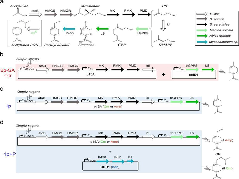
The figure below summarize the construction.
Biosynthetic pathway of fragrance and construction of our model
By analysing the different reaction in pathway above and using the equations of Michaelis-Menten, we obtain the system of ten equations below:
\[
\left\lbrace
\begin{array}{llllllllll}
\frac{d[acetyl-CoA]}{dt} &= - \frac{Vm1 [acetyl-CoA]}{Km1 + [acetyl-CoA]} \\
\frac{d[acetoacetyl-CoA]}{dt} &= \frac{Vm1 [acetyl-CoA]}{Km1 + [acetyl-CoA]} - \frac{Vm2 [acetoacetyl-CoA]}{Km2 + [acetoacetyl-CoA]} \\
\frac{d[HMG-CoA]}{dt} &= \frac{Vm2 [acetoacetyl-CoA]}{Km2 + [acetoacetyl-CoA]} - \frac{Vm3 [HMG-CoA]}{Km3 + [HMG-CoA]} \\
\frac{d[Mevalonate]}{dt} &= \frac{Vm3 [HMG-CoA]}{Km3 + [HMG-CoA]} - \frac{Vm4 [Mevalonate]}{Km4 + [Mevalonate]} \\
\frac{d[MevalonateP-5]}{dt} &= \frac{Vm4 [Mevalonate]}{Km4 + [Mevalonate]} - \frac{Vm5 [MevalonateP-5]}{Km5 + [MevalonateP-5]} \\
\frac{d[5-pyroP-MevalonateP]}{dt} &= \frac{Vm5 [MevalonateP-5]}{Km5 + [MevalonateP-5]} - \frac{Vm6 [5-pyroP-MevalonateP]}{Km6 + [5-pyroP-MevalonateP]} \\
\frac{d[IPP]}{dt} &= \frac{Vm6 \frac{[5-pyroP-MevalonateP]}{2}}{Km6 + \frac{[5-pyroP-MevalonateP]}{2}} - \frac{Vm7 \frac{[IPP]}{2}}{Km7 + \frac{[IPP]}{2}} - \frac{Vm8 \frac{[IPP]}{2}}{Km8 + \frac{[IPP]}{2}} \\
\frac{d[DMAPP]}{dt} &= \frac{Vm6 \frac{[5-pyroP-MevalonateP]}{2}}{Km6 + \frac{[5-pyroP-MevalonateP]}{2}} + \frac{Vm7 \frac{[IPP]}{2}}{Km7 + \frac{[IPP]}{2}} - \frac{Vm8 \frac{[DMAPP]}{2}}{Km8 + \frac{[DMAPP]}{2}} \\
\frac{d[GPP]}{dt} &= \frac{Vm7 \frac{[IPP]}{2}}{Km7 + \frac{[IPP]}{2}} + \frac{Vm8 \frac{[DMAPP]}{2}}{Km8 + \frac{[DMAPP]}{2}} - \frac{Vm_f [GPP]}{Km_f + [GPP]} \\
\frac{d[Fragrance]}{dt} &= \frac{Vm_f [GPP]}{Kmf + [GPP]}
\end{array}
\right.
\]
where $Vm_f$ and $Km_f$ are constant relative to the Fragrance ie Limonene, Geraniol or Pinene.
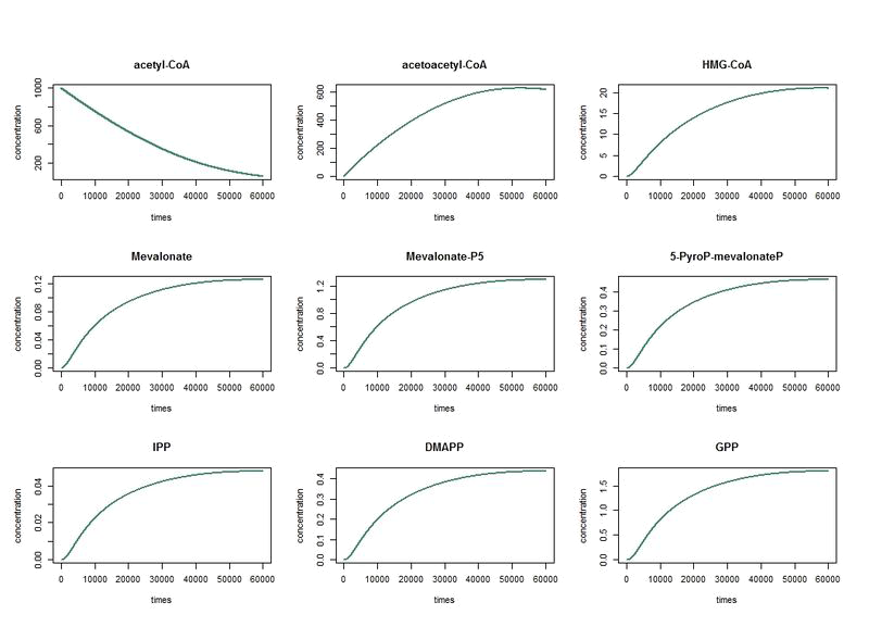
To solve these equation, we use the logiciel R and we obtain these following results for the production of Limonene, geraniol and pinene:
The differents constant are obtained via Brenda enzyme database: http://www.brenda-enzymes.org/
Results
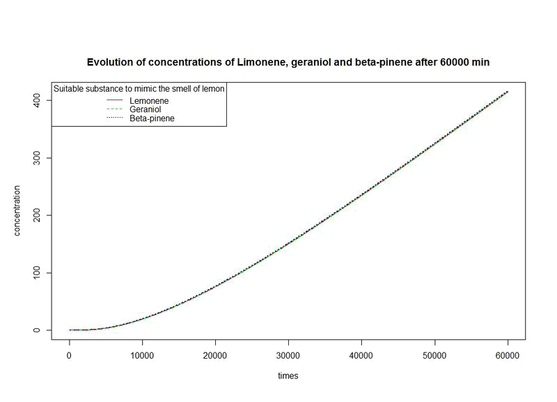
The nine first equations of our model remain the same regarding the evolution of limonene, pinene or geraniol. That's why we have put them in only one figure. The representations describe the evolutions over a long period of time.
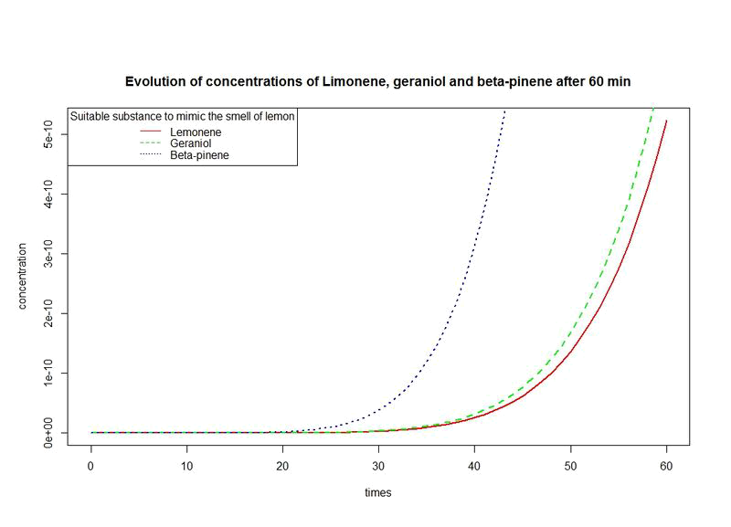
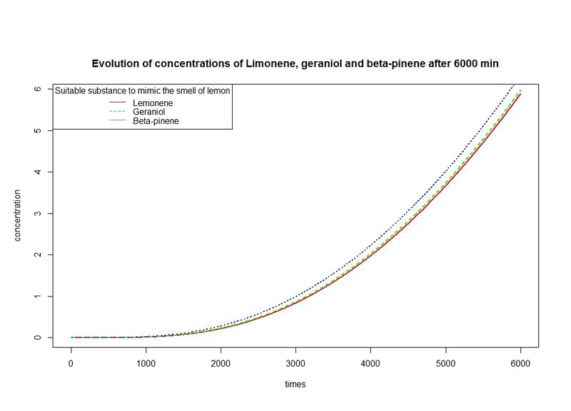
However, the production rates of limonene, geraniol and pinene are differents. By placing the evolutions of their concentrations in the same figure and for differents time sequences, we observe a kind of convergence of the three concentrations.
This means that after a while, limonene, geraniol and pinene have the same concentrations: a balance will thus settle. This phenomenon is represented by the images below where concentration are in µM (micromolar) and times in minute.
We will now establish a method to provide an answer to the question :
How to determine the right concentrations for the smell of lemon ?
De gustibus non est disputandum ! Similarly, there may be differences of opinion regarding odors. To avoid having considerations or philosophies built in vacuum, we will try to "quantify" or at least have a decision procedure works on the problematic identification of the "fragrance of lemon."
Let $L_t$ (resp. $G_t$ and $P_t$) be the concentration of limonene (resp. geraniol and pinene) at time t. We have access to this data through the work done previously.
We look for a time interval $[t_{d_n}, t_{f_n}]$ that will be considered as the region of "good smell" that is to say, times when the three concentrations take values close to perfect concentration to say we have a "good lemon scent". We note that perfect interval $[t_d, t_f]$: $t_d$ and $t_f$ are unknow. We will estimate them with $(t_{d_n})_{ n \in \mathbb{N} }$ and $(t_{f_n})_{ n \in \mathbb{N} }$.
Experimental design
We choose randomly $n$ individuals and let evolve the process $(L_t)_t$, $(G_t)_t$ and $(P_t)_t$. Thus, for an individual $ i \in \{1, \cdots, n \} $ fixed, he may decide times $[t_{d_i}, t_{f_i}]$ when he feels a lemon scent. For this individual, good concentrations will therefore be $L_{d_i}$, $G_{d_i}$ and $P_{d_i}$. This gives:
\[ \text{for individual 1, we have the interval } [t_{d_1}, t_{f_1}]. \]
\[ \text{For individual 2, we have the interval } [t_{d_2}, t_{f_2}]. \]
\[ \cdots \]
\[ \cdots \]
\[ \text{For individual j, we have the interval } [t_{d_j}, t_{f_j}]. \]
\[ \cdots \]
\[ \cdots \]
\[ \text{For individual n, we have the interval } [t_{d_n}, t_{f_n}]. \]
When $n$ becomes large and under assumptions of application of the famous law of large numbers, we have :
$$ \frac{1}{n} \sum_{i = 1}^{n} t_{d_i} \longrightarrow E[t_{d_1}] $$ $$ \frac{1}{n} \sum_{i = 1}^{n} t_{f_i} \longrightarrow E[t_{f_1}] $$
Thus from the data collected, we will have access to a functional of the perfect interval for smelling the lemon.
[1] Gilles Camus, La cinétique des enzymes michaeliennes et l'équation de Michaelis-Menten, 22 novembre 2012.
[2] Jorge Alonso-Gutierrez, Rossana Chan, Tanveer S.Batth, Paul D.Adams, Jay D.Keasling, Christopher J.Petzold, Taek Soon Lee, Metabolic engineering of Escherichia coli for limonene and perillyl alcohol production.
[3] Karline Soetaert, Thomas Petzoldt and R. Woodrow Setzer, Solving Differential Equations in R .
 "
"


