Team:Colombia/Stochastic
From 2014.igem.org
(Difference between revisions)
| Line 1: | Line 1: | ||
{{Http://2014.igem.org/Team:Colombia}} | {{Http://2014.igem.org/Team:Colombia}} | ||
| + | |||
| + | <html> | ||
<div class="span11" style="text-align: justify;"> | <div class="span11" style="text-align: justify;"> | ||
<center> | <center> | ||
| Line 15: | Line 17: | ||
It is well known that we can simulate this kind of molecular dynamics as stochastic processes. In particular, such events will be simulated as Markovian random walk in N dimension, where N represents the number of substances involved. | It is well known that we can simulate this kind of molecular dynamics as stochastic processes. In particular, such events will be simulated as Markovian random walk in N dimension, where N represents the number of substances involved. | ||
| - | <i> | + | <center><i> |
“…For “ordinary” chemical systems in which fluctuations and correlations play no significant role, the method stands as an alternative to the traditional procedure of numerically solving the deterministic reaction rate equations. For nonlinear systems near chemical instabilities, where fluctuations and correlations may invalidate the deterministic equations, the method constitutes an efficient way of numerically examining the predictions of the stochastic master equation. Although fully equivalent to the spatially homogeneous master equation, the numerical…” (Gillespie 1976) | “…For “ordinary” chemical systems in which fluctuations and correlations play no significant role, the method stands as an alternative to the traditional procedure of numerically solving the deterministic reaction rate equations. For nonlinear systems near chemical instabilities, where fluctuations and correlations may invalidate the deterministic equations, the method constitutes an efficient way of numerically examining the predictions of the stochastic master equation. Although fully equivalent to the spatially homogeneous master equation, the numerical…” (Gillespie 1976) | ||
| - | </i> | + | </i></center> |
| - | + | ||
| - | + | ||
| Line 28: | Line 28: | ||
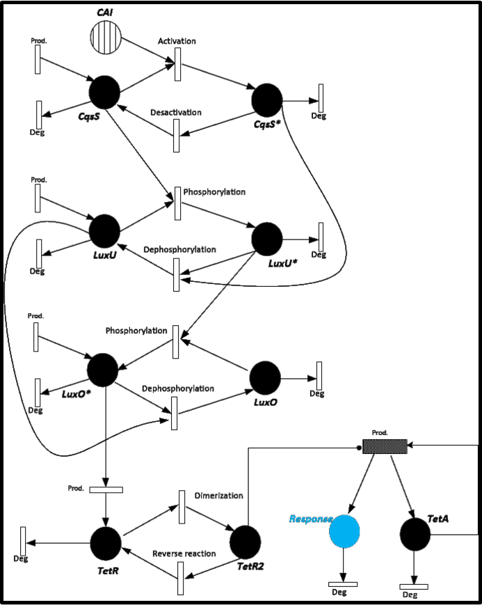
To give you an idea of how does our system works and how will be the events related, we present a Stochastic Petri Net. In Figure 1 we can appreciate the different molecules species interacting between them or undergoing process such as degradation or production.<br> | To give you an idea of how does our system works and how will be the events related, we present a Stochastic Petri Net. In Figure 1 we can appreciate the different molecules species interacting between them or undergoing process such as degradation or production.<br> | ||
| - | + | </html> | |
[[File:Colombia_PetriNet.png|left|600px]] | [[File:Colombia_PetriNet.png|left|600px]] | ||
| + | <html> | ||
<center> <b>Figure 1</b> </center> | <center> <b>Figure 1</b> </center> | ||
<br> | <br> | ||
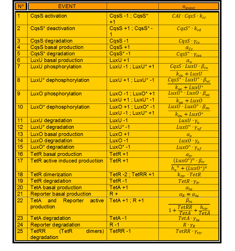
In this case, we have 24 different possible events to take into account. (Table 1) | In this case, we have 24 different possible events to take into account. (Table 1) | ||
| + | </html> | ||
[[File:Colombia_TableEst1.jpg|left|600px]] | [[File:Colombia_TableEst1.jpg|left|600px]] | ||
| + | <html> | ||
| + | |||
<center> | <center> | ||
| Line 52: | Line 56: | ||
Let’s define | Let’s define | ||
| + | </html> | ||
[[File:Col_Ecu2.png|left|600px]] | [[File:Col_Ecu2.png|left|600px]] | ||
| + | <html> | ||
<br> | <br> | ||
Now divide [0,1] in 25 interval such that (Figure 2) | Now divide [0,1] in 25 interval such that (Figure 2) | ||
| - | + | </html> | |
[[File:Col_Ecu3.png|left|600px]] | [[File:Col_Ecu3.png|left|600px]] | ||
| + | <html> | ||
<br> | <br> | ||
| - | + | </html> | |
[[File:Col_Img4.png|left|600px]] | [[File:Col_Img4.png|left|600px]] | ||
| + | <html> | ||
<center> <b>Figure 2</b> </center> | <center> <b>Figure 2</b> </center> | ||
Revision as of 03:46, 18 October 2014
Stochastic Model.
In this case, we have 24 different possible events to take into account. (Table 1)
The time τ between events is calculated by: [[File:Col_Ecu1.jpg|left|600px]]
Which event will occur is calculated by using another random number R between 0 and 1 in the following way:
Let’s define
Now divide [0,1] in 25 interval such that (Figure 2)
The size of the ith interval depends on the value of n_i.
The event that will occur is the one that correspond to in which interval is located the random number R.
Results
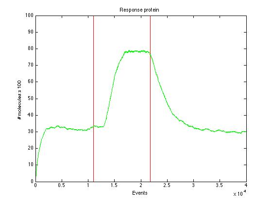
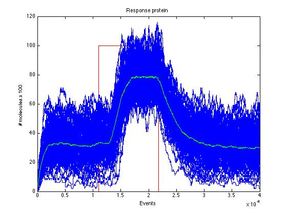
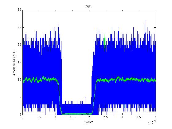
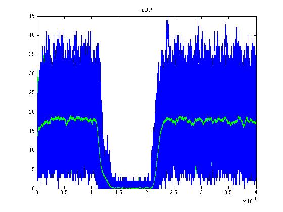
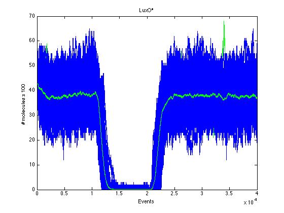
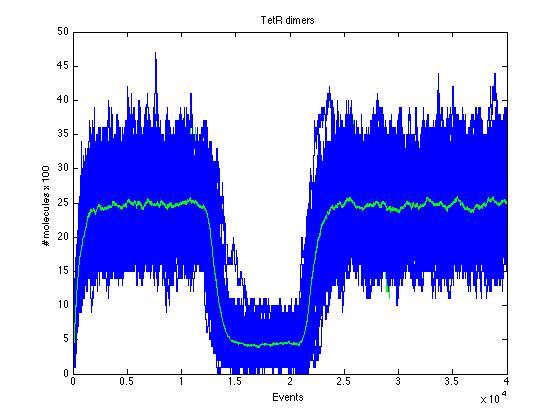
Here we present a graphic for each molecule species involved in our system and how it responds to the presence of CAI-1 in the environment. The red line in the Figure 3 represents the amount of CAI-1 molecules in the environment.The blue lines represent the behavior of each cell and the green line presents the mean behavior of the total population.
As we can see CqsS and CqsS* have oposing (complementary) behaviors as we would expect this can be seen in figures 5 and 6 Same goes for LuxU and LuxU*, and LuxO and LuxO* in figures 7, 8, 9 and 10 respectively
Also in figure 11 can be seen how such a small change in TR has a drastic effect in the TR dimer.
 "
"


