Background: Growth Curve
A growth curve for a population of bacteria illustrates some of the dynamics that affect the population size over time.
Four distinct phases are recognized:
The lag phase:
The curve remains at a plateau. During this time, bacteria adapt to their new environment, store nutrients and prepare for binary fission.
The logarithmic phase:
This phase is also called the exponential growth phase: the population of bacteria enters an active stage of growth, the mass of each cell increases rapidly, and the number of bacteria doubles.
The stationary phase:
At this stage reproductive and death rates equalize, the population enters another plateau.
Models and mathematic equations
Three well known growth models (Logistic, Gompertz, and Richartz)are used in this work. Characteristic model parameters (such as lag phase (λ), maximal growth rate (µ-max slope), stationary phase (A-max growth value)) are derived from our experimental data. Bootstrap and cross-validation techniques are used for estimating confidence intervals of
all derived parameters.
The aim is to integrate the experimental data into different growth models and to compare the models using statistical methods (AIC and maximum likelihood were used). We believe, and many scientists do, that model selection is the most important part in model-experiment based research-The right data with the right model.
Logistic Model:
$$\begin{align}
y(t)&=\frac{A}{1+\exp\left(\frac{4\mu}{A}(\lambda-t)+2\right)}
\end{align}$$
Gompertz Model:
$$\begin{align}
y(t)&=A.\exp\left[-\exp\left(\frac{\mu.\exp(1)}{A}(\lambda-t)+1\right)\right]
\end{align}$$
Richartz Model:
\begin{align}
y(t)&=A.\left[1+\nu\exp\left(1+\nu+\frac{\mu}{A}(1+\nu)^{1+1/\nu}(\lambda-t)\right)\right]^{-1/\nu}
\end{align}
$\nu$ is a shape parameter (in the richartz model only)
pH model
Existed model is
$$\begin{align}
\frac{dpH}{dP}&=k(pH-pH_{min})
\end{align}$$
However, this model is not appropriate for our experimental data; we used linear regression model instead.
$$pH=\alpha + \beta OD +\epsilon$$
where $\epsilon$ is a random error or noice (which helps to capture a measurement error and other unknown factors). And it is assumed to be Gaussian (normal distribution function), $\epsilon = N(\theta,\sigma^{2})$, with mean $\theta$ and constant variance $\sigma^{2}$. $\alpha$ and $\beta$ are model parameters.
Result and model validation
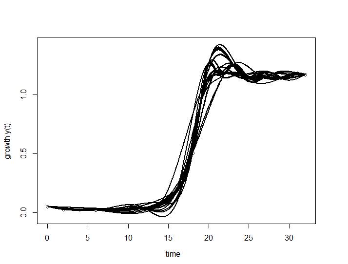
Figure 1: Simulation results of the growth curve
Our experimental data are implemented in the three proposed models. AIC is used to measure the performance of the models and the result shows that Logistic and Richartz models are approximately the same, but slightly different from Gompertz. However, using 95% confidence interval all of them are appropriate to fit the given data.
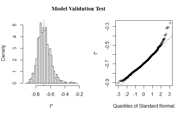
Figure 2: Shows validation test(t*) for the fitted model
The validation test (plot of the residuals), as Figure 2, shows that the simulation result obtained from bootstrap samples is suitable to estimate the model parameters.
Using our experimental data as initials samples, we applied Bootsrap statistical to sample empirical data. The simulated result is presented as Figure (1). And, the estimated model parameters (mu(µ), lamda(λ), A) are summarized as Table 1.
$$\text{Table 1: Estimated Model Parameter}$$
-------------------------------------------
           mu          lamda         A
===========================================
Lower     0.294        16.041       1.155
Mean      0.384        16.456       1.187
Upper     0.474        16.871       1.220
Std       0.046        0.212        0.016
-------------------------------------------
Integral value: 16.622
-------------------------------------------
From the result on table $1$, the $lower$ and $upper$ values are the estimated confidence intervals of the corresponding parameters. $Std$-standard deviation) and $mean$-average values are obtained from the bootstrap samples. These results are used in the proposed three growth models. After the approprate models are selected (in our case, the three proposed models are equally approprate), the parameters are taken as an intial values for the interaction model; which is used to study the growth of S.mutant in the presence of other species(see competition model).
$$\text{Table 2: Analysis of Regression Model}$$
==============================================================
Estimated parametrs:        |  Statistical Tests:
Intercept (alpha)=7.6074    |  R-squared= 0.9135
OD (beta)=-2.0365           |  p-value=6.228e-14
--------------------------------------------------------------
F-statistic=254.6
===============================================================
Using the table 2 result, the pH model can be estimated as: $pH=7.61 - 2.04 OD$
There is a strong linear correlation between pH and OD (R=0.9135, F=254.5, P.value $<$0.05). The coefficient value indicates that for every additional unit in OD we can expect pH to decrease by an average of 2.04. For examples: if the OD=1, pH is expected to be (pH=7.61 - 2.04(1))=5.57. The red fitted line graphically shows the same information.
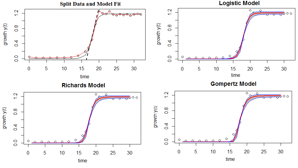
Figure 3: Shows model comparison-the shaded regions indicate a 95% confiden interval of the model fits (bold lines)
If we move left or right along the x-axis by an amount that represents a one unit change in OD, the fitted line falls by 2.04 units. If the fitted line was flat (a slope coefficient of zero), the expected value for pH would not change no matter how far up and down the line you go. So, the low p-value ($\leq$ 0.05) suggests that the slope is not zero, which in turn suggests that changes in the predictor variable(OD) are associated with changes in the response variable (pH). R-squared is a statistical measure of how close the data are to the fitted regression line. It is also known as the coefficient of determination. It is the percentage of the response variable variation that is explained by a linear model. In this case, R-square =0.9135 shows that 91.35% of the pH variation is explained by OD, and the remain 8.65 can be explained by other factors that are not considered in the regression model.

Figure 4: ph vs OD with 95% confident interval
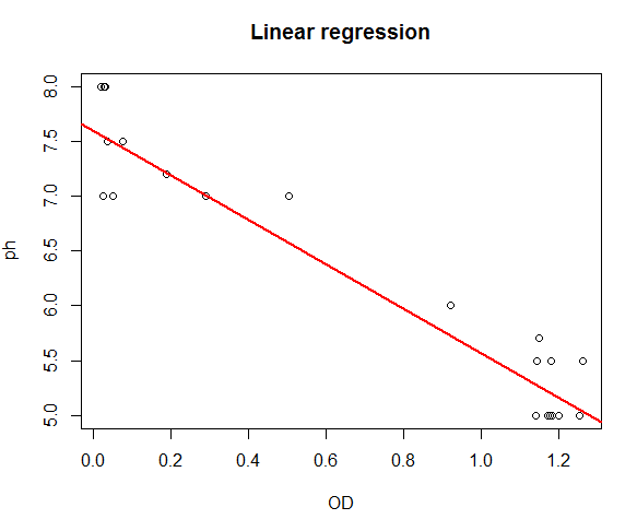
Figure 5: Model Fit
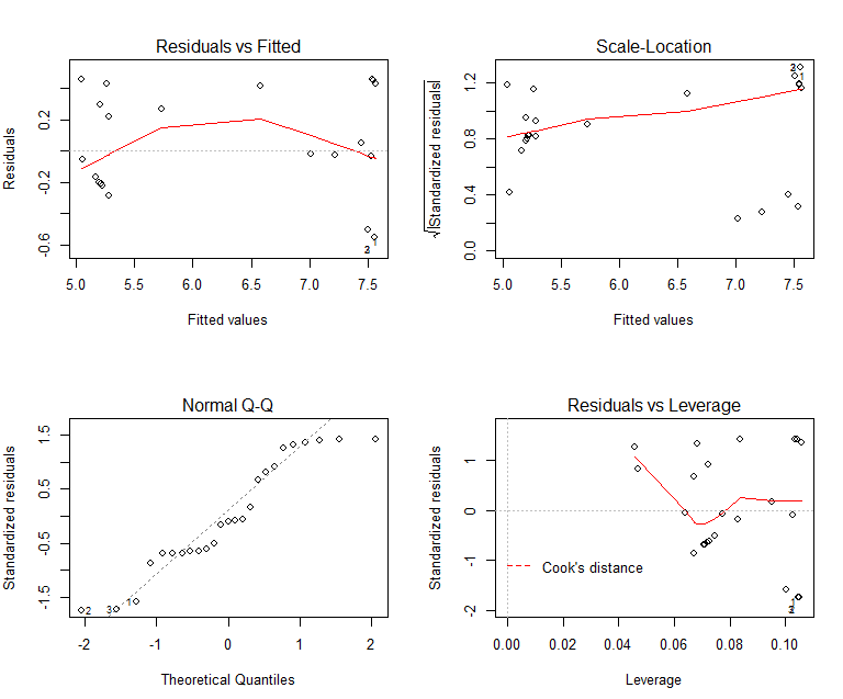
Figure 6: Validation Test
 "
"