Team:LMU-Munich/Project/Modeling
From 2014.igem.org
Hoerldavid (Talk | contribs) |
Hoerldavid (Talk | contribs) |
||
| Line 70: | Line 70: | ||
=== Implementation === | === Implementation === | ||
| + | |||
| + | <html> | ||
| + | </section> | ||
| + | </div> | ||
| + | <section class="accordion"> | ||
| + | <div> | ||
| + | <input id="model-ct-source" name="model-accord" type="checkbox" /> | ||
| + | <label for="model-ct-source">Source</label> | ||
| + | <article class="ac-small"> | ||
| + | </html> | ||
| + | |||
| + | |||
| + | |||
| + | <html></article></div></div></html> | ||
We implemented the model in C++, making extensive use of the ''Boost'' libraries for numerical integration, among other things. In addition, | We implemented the model in C++, making extensive use of the ''Boost'' libraries for numerical integration, among other things. In addition, | ||
Revision as of 15:30, 17 October 2014
Modeling
Lorem ipsum dolor sit amet, consetetur sadipscing elitr, sed diam nonumy eirmod tempor invidunt ut labore et dolore magna aliquyam erat, sed diam voluptua. At vero eos et accusam et justo duo dolores et ea rebum. Stet clita kasd gubergren, no sea takimata sanctus est Lorem ipsum dolor sit amet. Lorem ipsum dolor sit amet, consetetur sadipscing elitr, sed diam nonumy eirmod tempor invidunt ut labore et dolore magna aliquyam erat, sed diam voluptua. At vero eos et accusam et justo duo dolores et ea rebum. Stet clita kasd gubergren, no sea takimata sanctus est Lorem ipsum dolor sit amet.
Chemotaxis
Motivation
To stay true to its title 'pathogen-hunting microbe', BaKillus should ideally be able to swim towards its prey via chemotaxis. However, the ability to react to an AIP- or CSP-gradient requires the introduction of a chimeric receptor into Bacillus subtilis. Chemotaxis receptors are quite complex and can, for example, take different methylation states to allow for attenuation of the chemotactic response. This complexity puts the construction of a custom receptor beyond the scope of an iGEM project.
To evaluate how a hypothetical chemotactic BaKillis would act in an experimental setting, we developed a model to simulate the movement of chemotactic hunters in response to an attractant gradient produced by a growing colony of prey bacteria.
Overview
Our multi-scale hybrid model essentially consists of 3 components: growth of prey bacteria (algebraic model), diffusion of attractant molecules (spatial partial differential equation) and chemotactic behavior of the hunter bacteria (stochastic spatial agent model coupled to differential equations for internal state with a stochastic driving force). All these processes take place in a defined geometric space (representing, for example, a microfluidic device). The experimental scenario we wish to capture in our model is the following: a colony of prey bacteria is spotted onto the arena, growing in place and producing attractant molecules. A fixed population of hunter bacteria is placed into the arena as well. Their reaction (biased movement) to the building attractant gradient is what we seek to observe.
Growth of prey
The prey bacteria will grow on a population level, according to a logistic growth curve with explicit solutions (ref!):
\[ y = ln \frac{N}{N_0} = \frac{A}{1 + e^{\frac{4\mu_m}{A} (\lambda - t) + 2}}\]
Here, \(N_0\) is the population size at \(t = 0\), \(A = ln \frac{N_\infty}{N_0}\) is the asymptote, \(\mu_m\) is the growth rate and \(\lambda\) the duration of the lag-phase.
Diffusion of attractants
The concentration of attractant molecules (\(c\)) in space changes according to a partial differential equation comprising diffusion, degradation and production by the prey bacteria.
\[ \frac{\partial c}{\partial t} = D\Delta c + p c_{prey} - a c\]
\(D\) is the diffusion coefficient, \(a\) is the degradation rate, \(p\) the rate of production and \(c_{prey}\) the concentration of prey/producer bacteria.
Chemotaxis
The chemotaxis of the hunter bacteria (BaKillus) is represented by an agent-based model adapted from [Matthäus ref]. Each bacterium has its own methylation and phosphorylation states of the chemotactic pathway which change according to a system of ordinary differential equations in response to attractant concentrations. In a classical 2-state model of bacterial chemotaxis, each bacterium will be in either running or tumbling state at each time point. In a running step, bacteria will swim forward in a straight line whereas in a tumbling step, they will change their direction by a random angle picked from a gamma distribution.
It should be noted that the model used here actually describes chemotaxis of E. coli. While the wiring of the chemotaxis pathway differs slightly, the same behavior is expected for B. subtilis . Therefore, we opted for the use of the better studied E. coli-model.
Implementation
We implemented the model in C++, making extensive use of the Boost libraries for numerical integration, among other things. In addition, we wrote gateway routines to allow handling of the model from a MATLAB script. This way, parameters can easily be changed and results can be visualized using the plotting functionality of MATLAB.
Initially, the arena in which chemotaxis should take place is defined as a polygon. An equally spaced 2-dimensional grid covering the polygon is created to store concentrations of prey bacteria and attractant molecules (fig. x). The area in which prey bacteria grow (a 'colony') is defined as a rectangle and their initial concentration is set.
[scheme of grid]
A desired number of virtual hunter bacteria are created at set spacial coordinates. Initially, these bacteria have a random orientation and their chemotactic pathway is inactive (methylation and phosphorylation levels are zero).
The model is then updated by defined time steps until a desired end time is reached.
At each time step, the number of prey bacteria in the colony is updated according to their logistic growth curve. The concentration of attractant molecules changes
according to the diffusion equation (see above). The Laplacian is discretized on the grid using a standard 5-point stencil (pseudocode??).
In each time step, the bacteria will update their chemotactic pathway (according to the system of differential equations) in response to the attractant concentration at their location (the mean of the nonnegative concentrations at the neighboring 4 grid nodes). Each bacterium will then swim forward (run) or change its orientation (tumble) dependent on the phosphorylation level of CheY.
Results & Discussion
Suicide Switch
For safety issues we want BaKillus to autoinduce apoptosis after successful completion of his task. This can be achieved by shutting down the production of resistance providing anti-toxin proteins. (see: Suicide-Switch) Still, BaKillus must produce sufficients amounts of toxins before inducing apotosis. Therefor, the negative feedback, which eventually stops production of anti-toxin must be sufficiently delayed to provide a sufficiently long timeframe for toxin production. However, as simple as this idea might sound in theory, robust practical implementation of such a module requires precise finetuning of the kinetics of the respective signalling cascade. In this model we tried to assess whether the inclusion of a secondary sigma factor could theoretically enhance the efficiency of the killing mechanism.
In the following we will compare two different models, one including only one sigma factor and one including two sigma factors. The models will be compared based on a fitness function which describes the difference between the toxin and antitoxin production over time. This should provide a measure of the effective number of produced molecules toxin molecules.
Basic Model
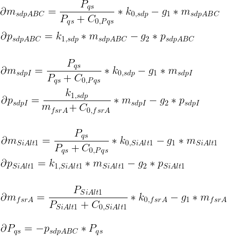
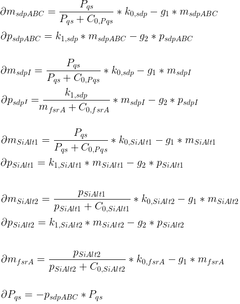
The basic model only contains one sigma factor. The system of differential equations was derived following the standard paradigm of gene expression including mRNA aswell as protein dynamics. Inhibitory and Promoting activity were modeled via hill kinetics.
Variables
| msdpABC: | Quantity of SdpABC mRNA |
| psdpABC: | Quantity of SdpABC proteins |
| msdpI: | Quantity of SdpI mRNA |
| psdpI: | Quantity of SdpI proteins |
| mSiAlt1: | Quantity of sigma factor mRNA |
| pSiAlt1: | Quantity of sigma factor proteins |
| mfsrA: | Quantity of FsrA mRNA |
| pfsrA: | Quantity of FsrA proteins |
| Pqs: | Quantity of QS proteins |
Inquired Parameters
| C0,Pqs: | Basic concentration of QS proteins |
| C0,psdpI: | Basic concentration of SdpI proteins |
| C0,fsrA: | Basic concentration of FsrA proteins |
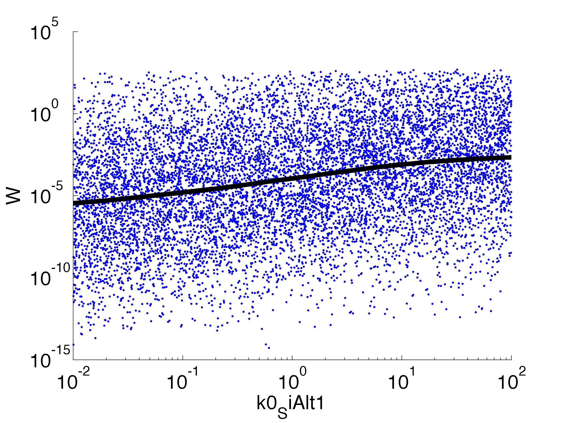
| k0,SiAlt1: | Transcription Rate of sigma factor |
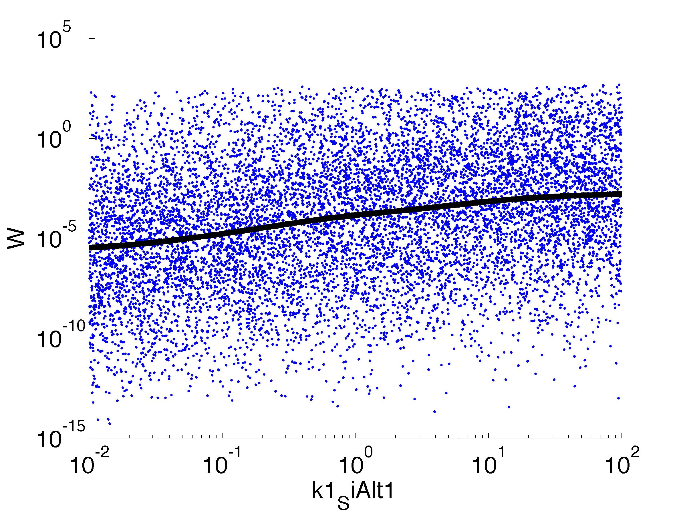
| k1,SiAlt1: | Translation Rate of sigma factor |
| C0,SiAlt1: | Basic concentration of sigma factor proteins |
| k0,fsrA: | Transcription Rate of FsrA |
| k1,fsrA: | Translation Rate of FsrA |
Fixed Parameters
In a first evaluation, the variation of following parameters were figured out to cause only insignificant variation of the model's fitness. Therefore they were keept at these specified values for all subsequent simulations:
| Degradation rate (g1) of mRNA: | 12 molecules per hour |
| Degradation rate (g2) of proteins: | 1 molecule per hour |
| Transcription rate (k0) of Sdp: | 7.2 per hour |
| Translation rate (k1) of SdpI & SdpABC: | 10 per hour |
% par0 = lhsdesign(10000,12);
par0 = rand(100000,12);
par = 10.^(4*par0 - 2); % Coveres range from 0.01 to 100

par(:,3) =12; % g1
par(:,5) =1; % g2
par(:,2) =0.12*60; % k0_sdp
par(:,4) =10; % k1_sdp

tout = linspace(0,10,100);
tic
for j = 1:size(par,1)
   [~,~,x,y] = simulate_RRE_cannibalism(tout,par(j,:));
    %figure
    %plot(tout,y)
    %legend('p_{p_sdpABC}','p_{p_sdpI}')

   W(j) = sum(y(:,1)-y(:,2));
end
toc

parname={'C0_Pqs','k0_sdp','g1','k1_sdp','g2','C0_p_sdpI', ...
'C0_fsrA','k0_SiAlt1','k1_SiAlt1','C0_SiAlt1','k0_fsrA','k1_fsrA'};

for k = [1,6,7,8,9,10,11,12]
  figure
  scatter(par(:,k),W',10,'filled')
  hold on

  [xx,ind]=sort(par(:,k));
  r = ksr(log10(xx),W(ind));

  plot(10.^r.x,smooth(r.f,10),'k-','LineWidth',5)
  set(gca,'Yscale','lin')
  set(gca,'Xscale','log')
  xlabel(parname{k})
  ylabel('W')
  saveas(gcf,['parameter_' parname{k}]);
  print('-depsc2','-r300',['parameter_' parname{k}])
end
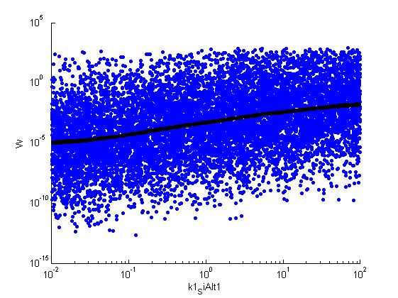
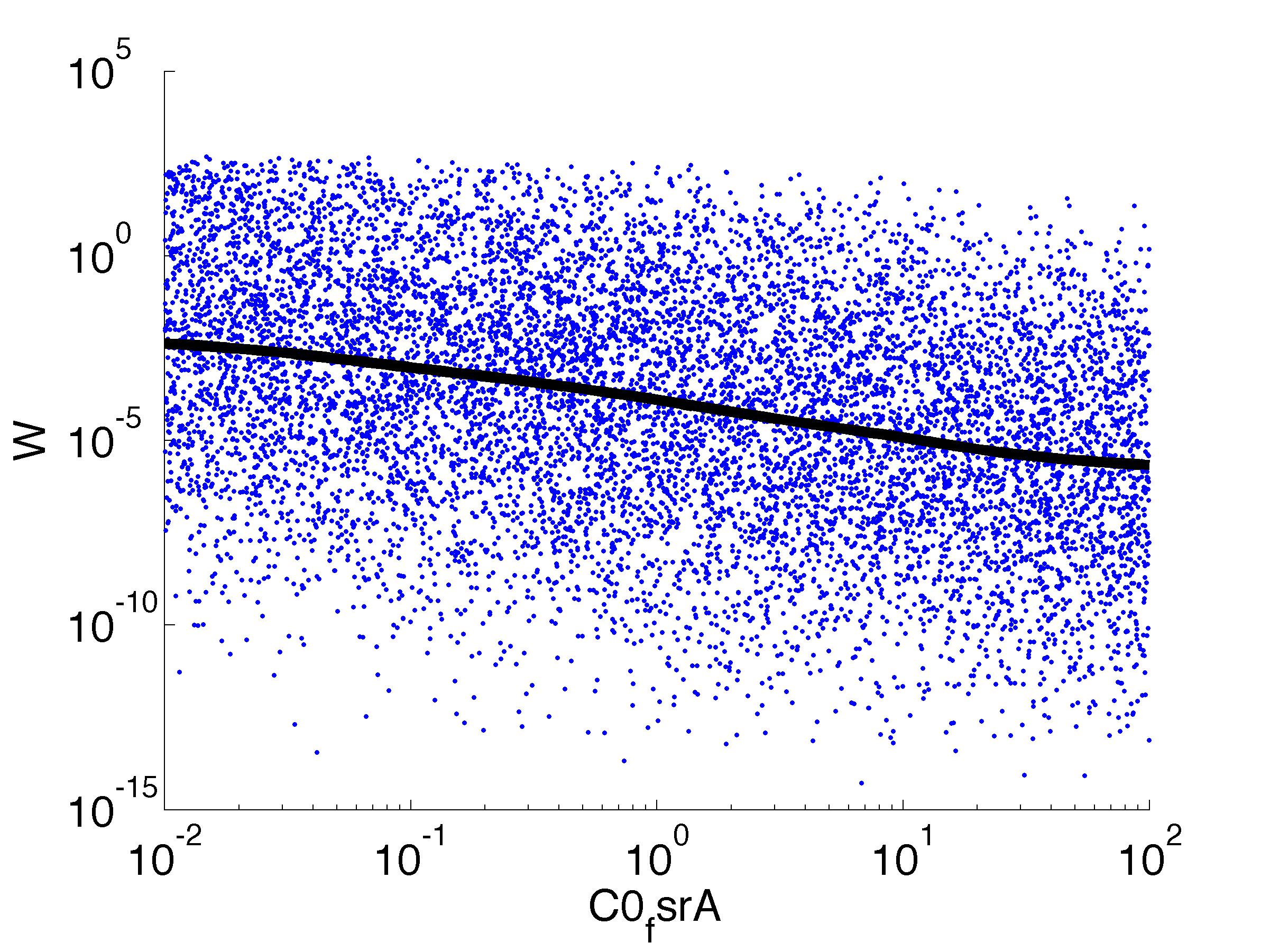
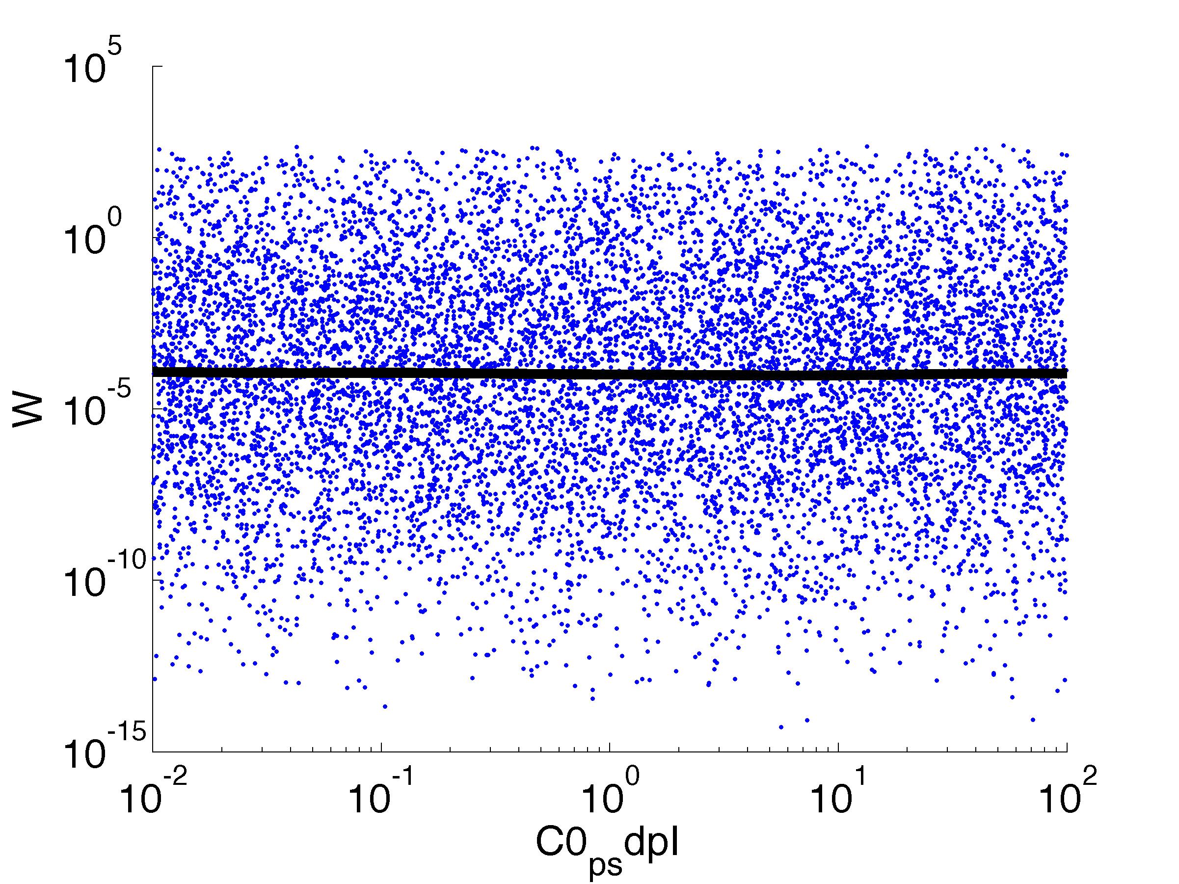
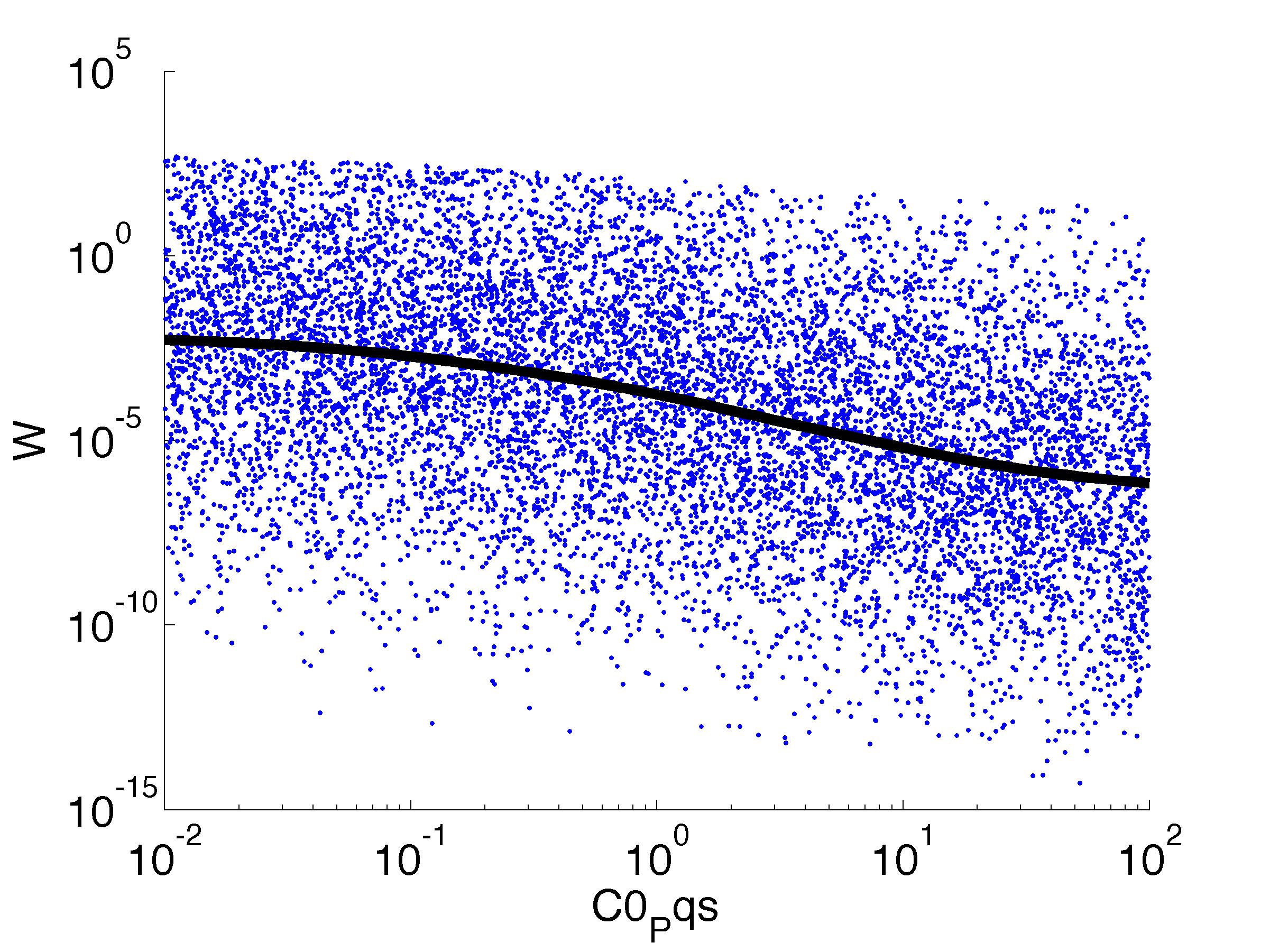
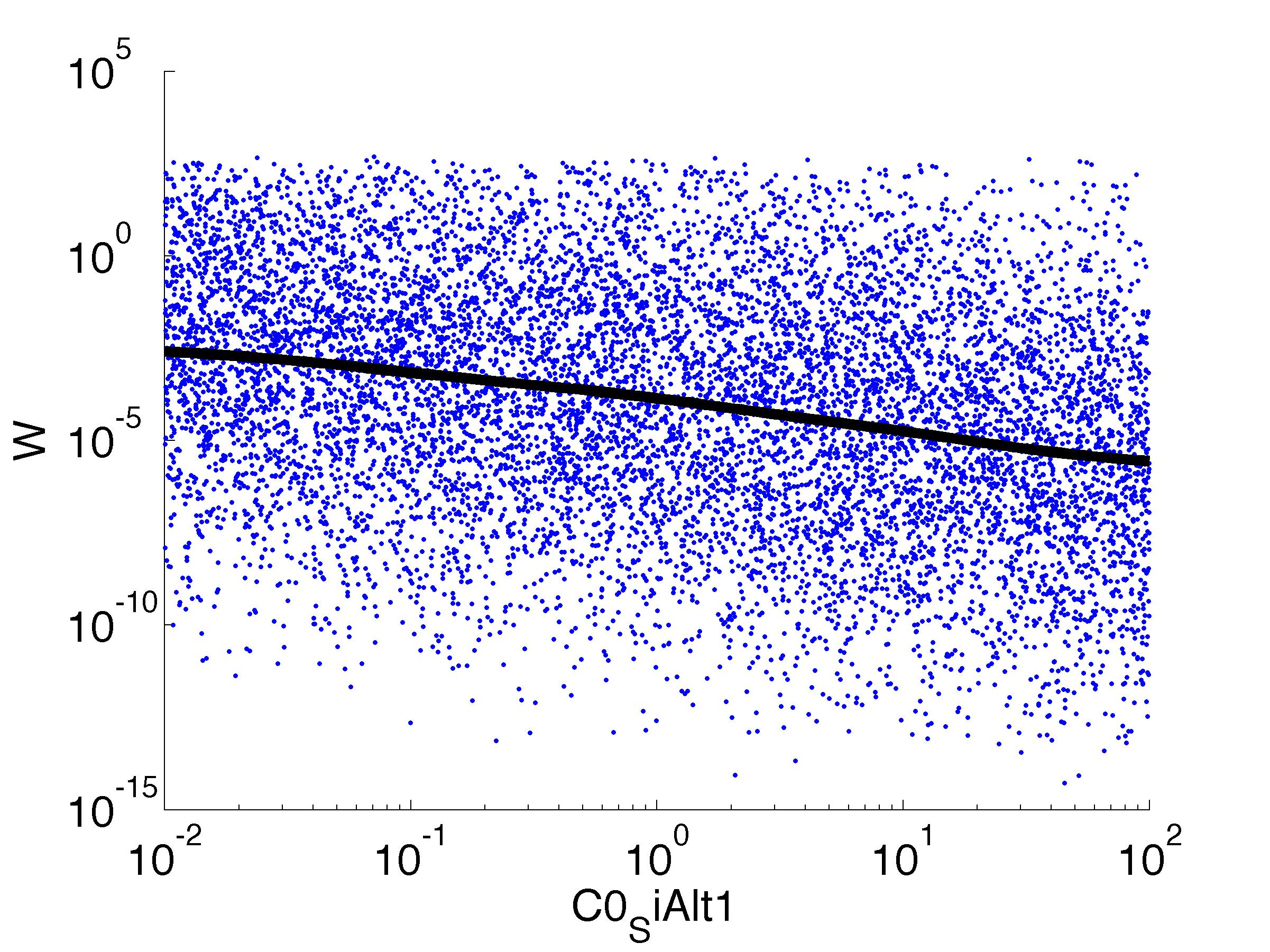
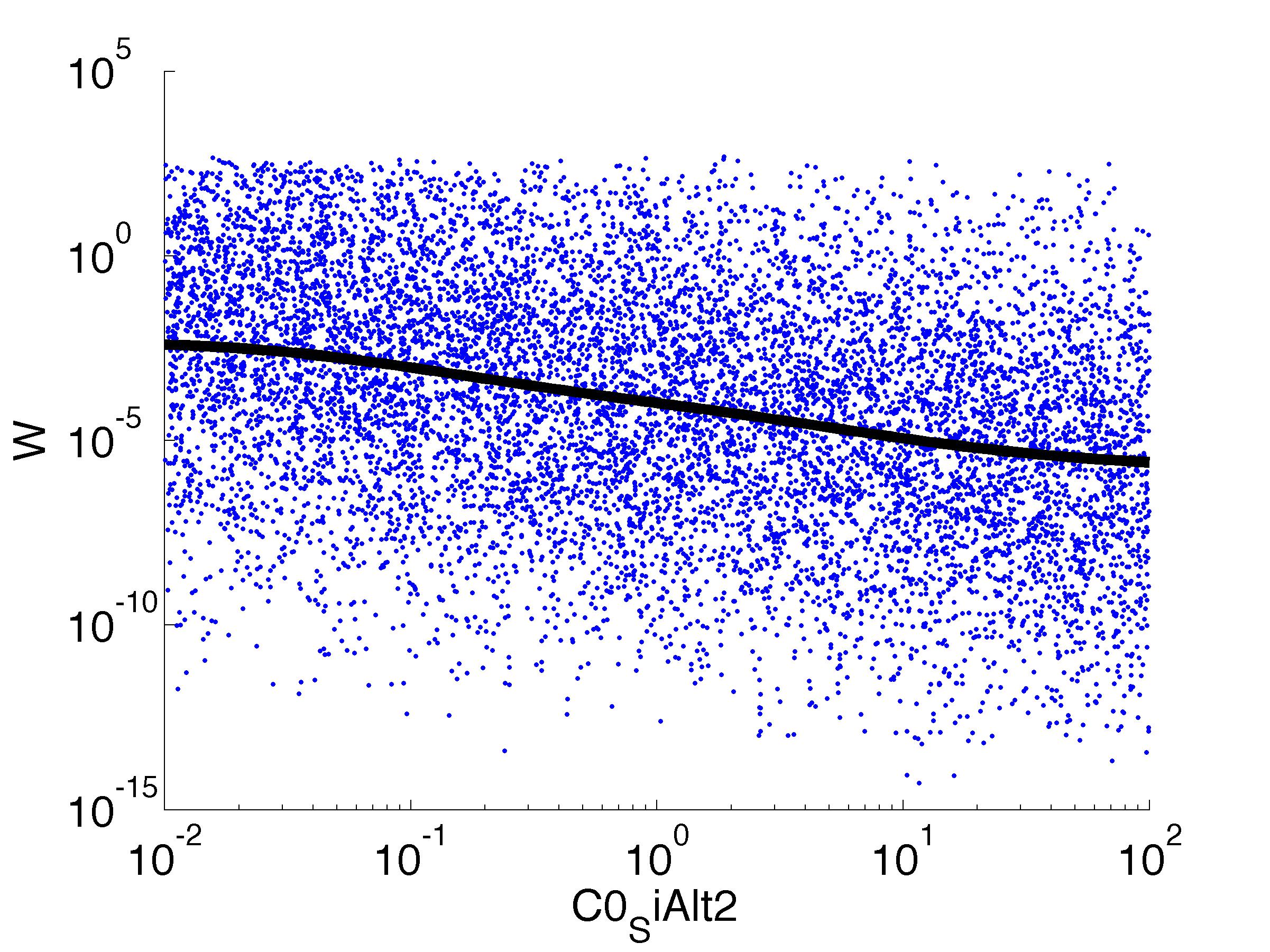
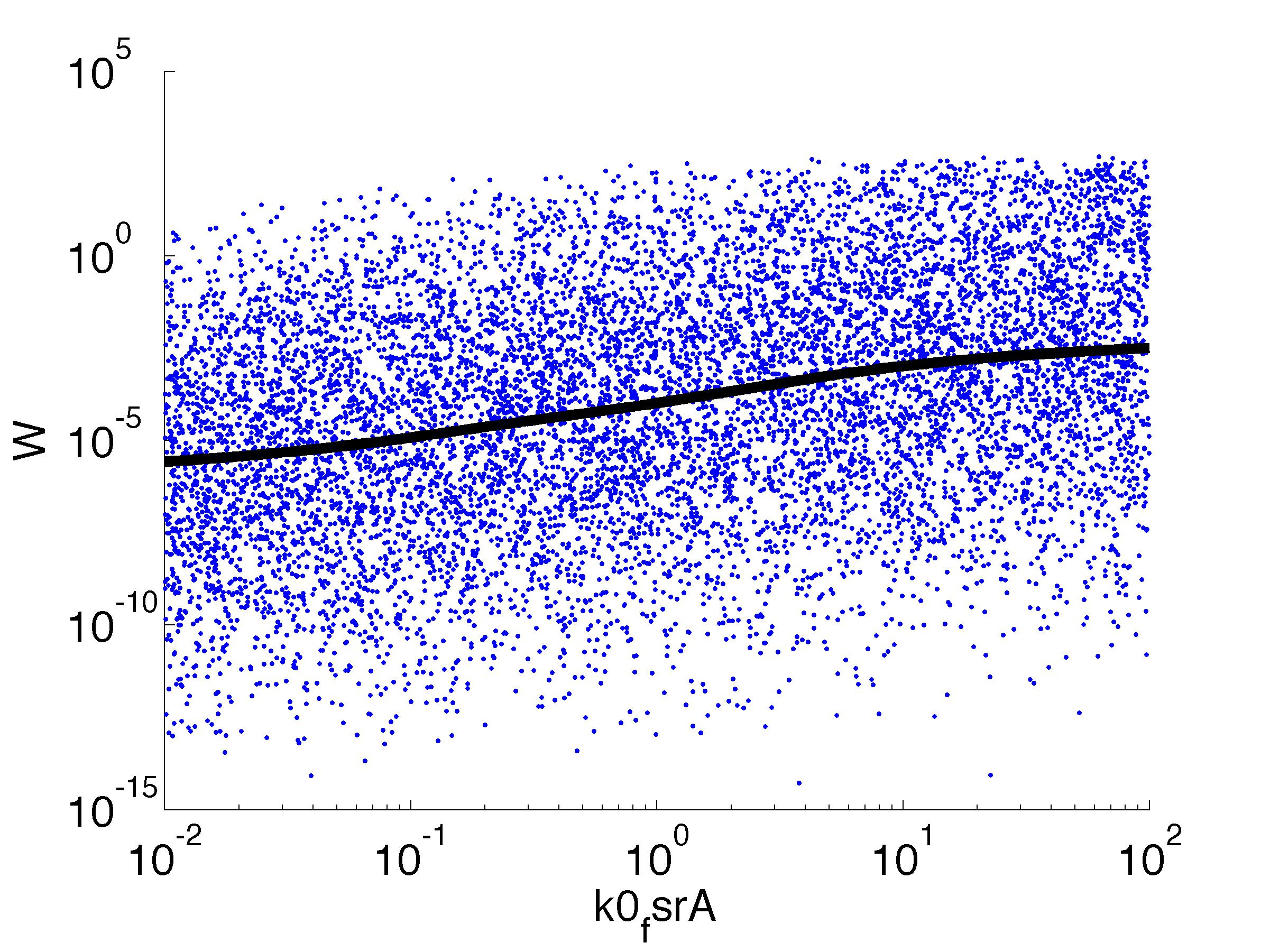
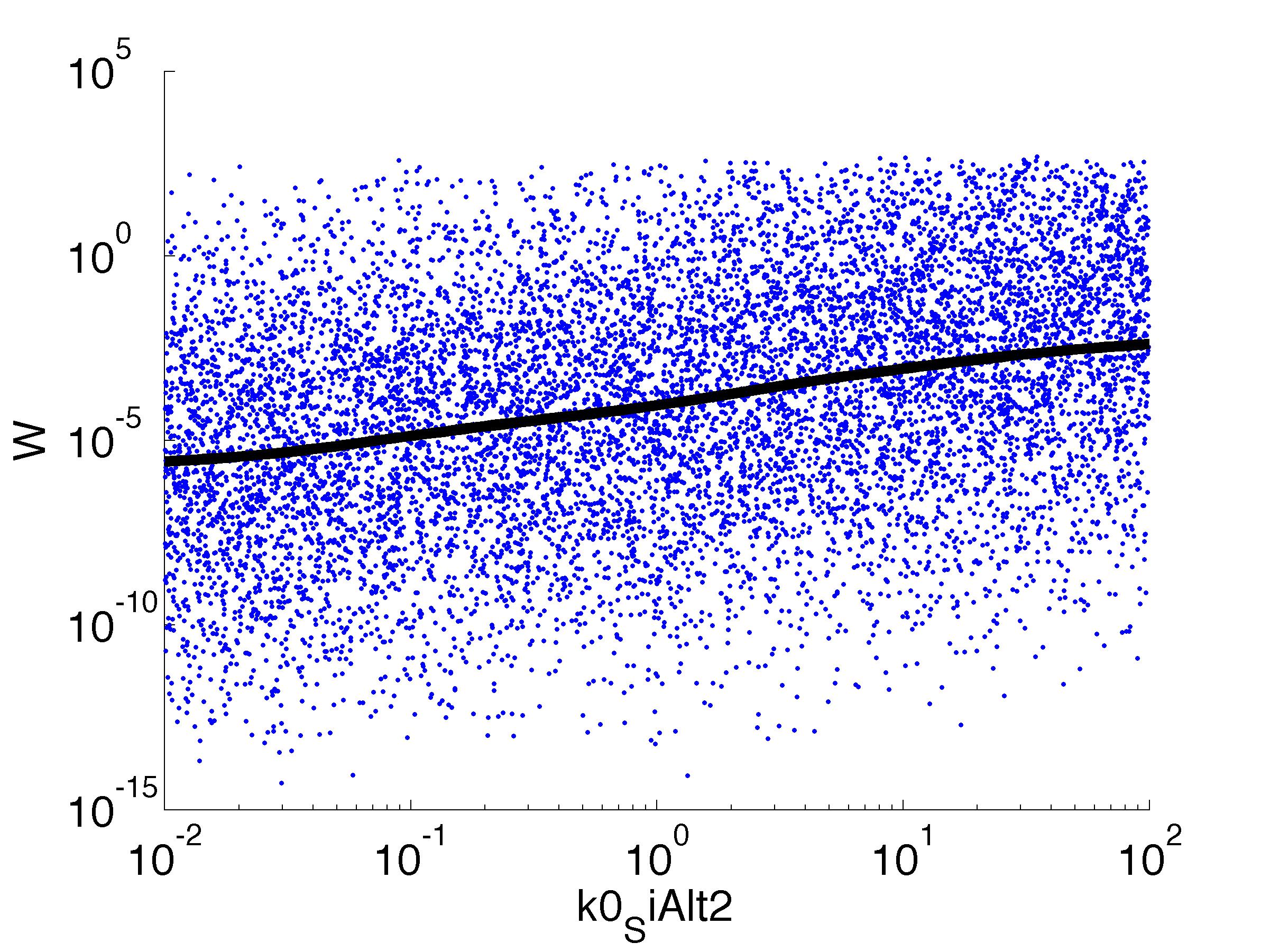
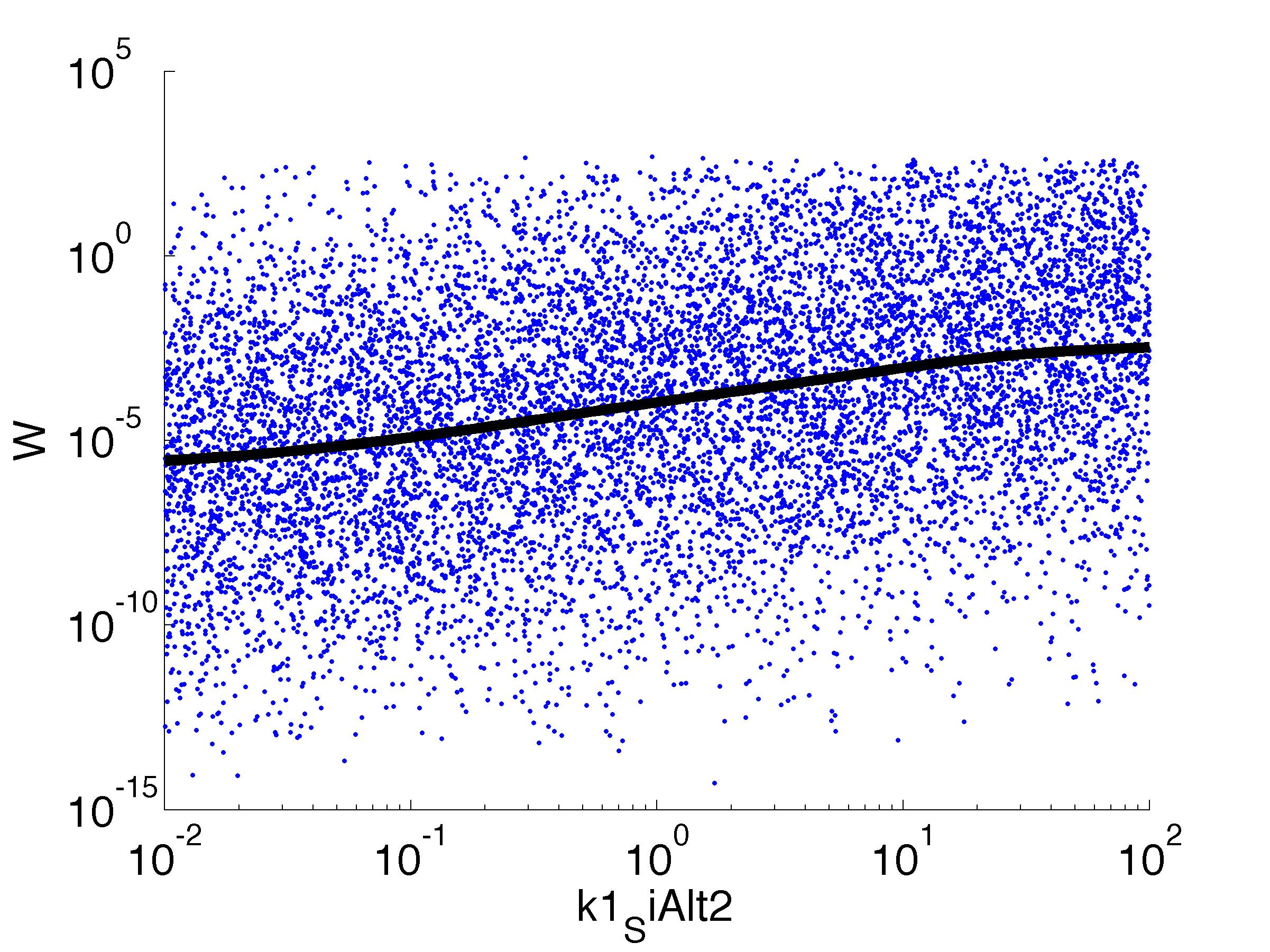
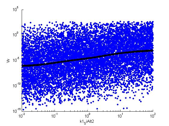
Fitness W
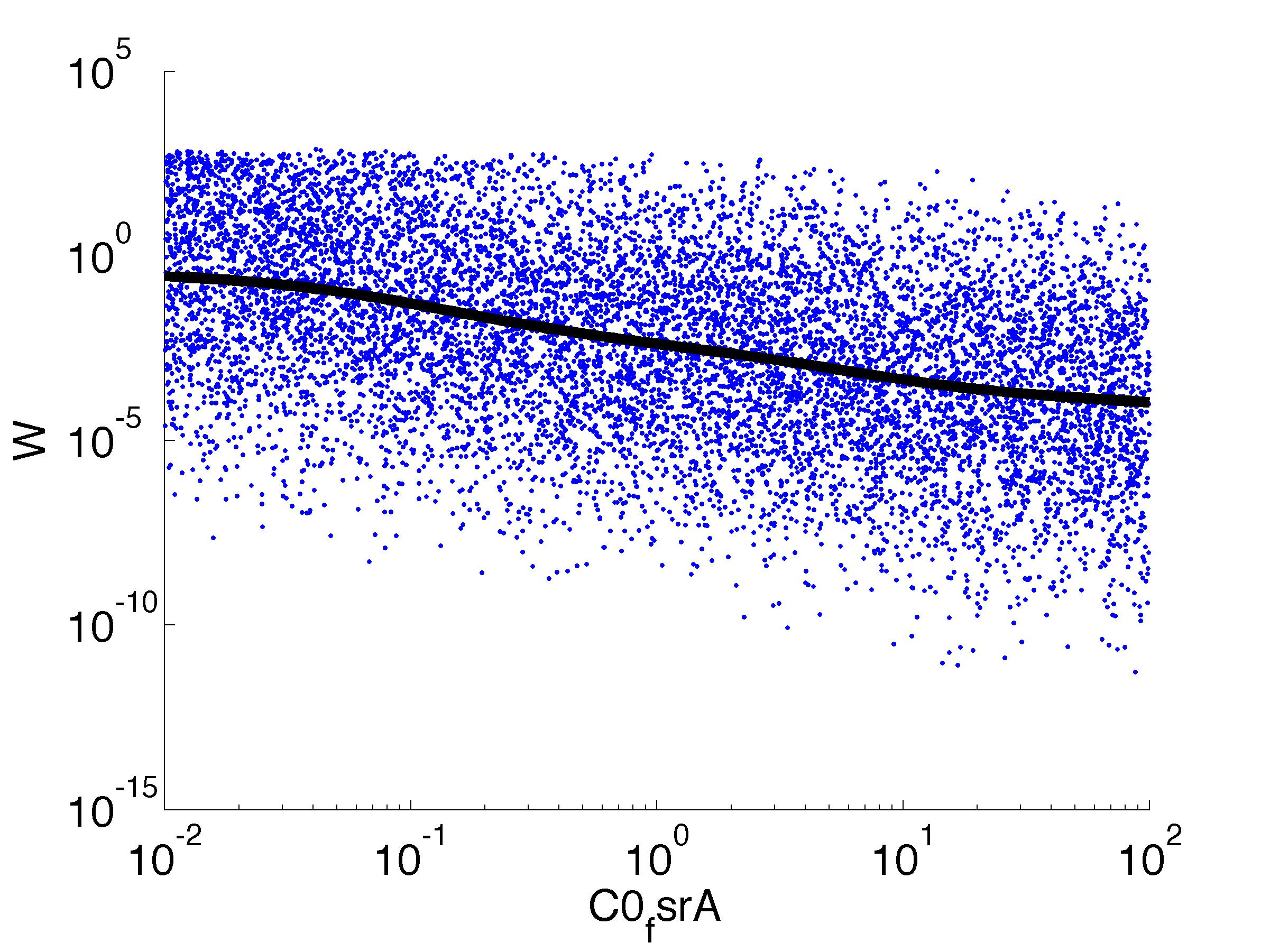
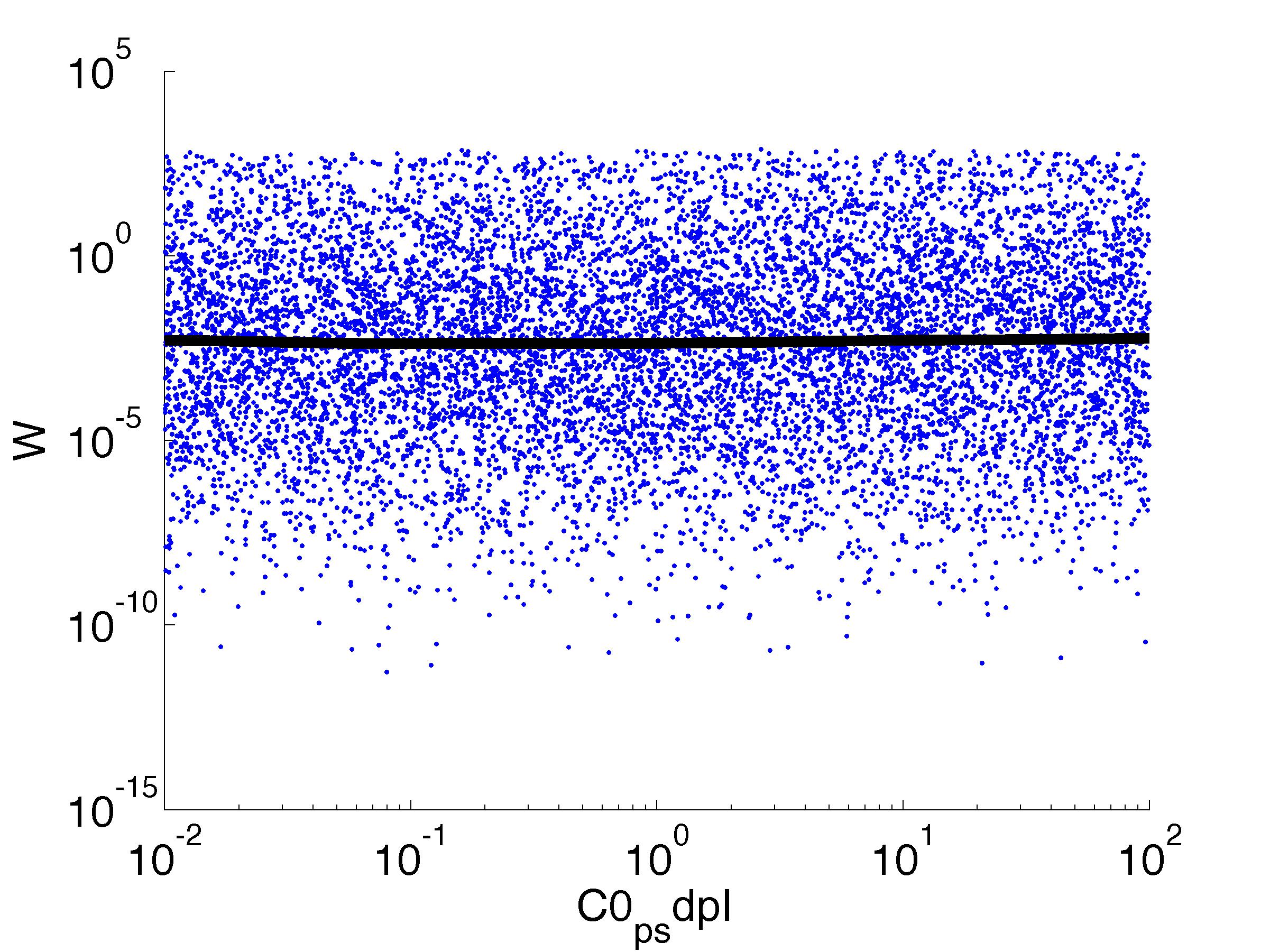
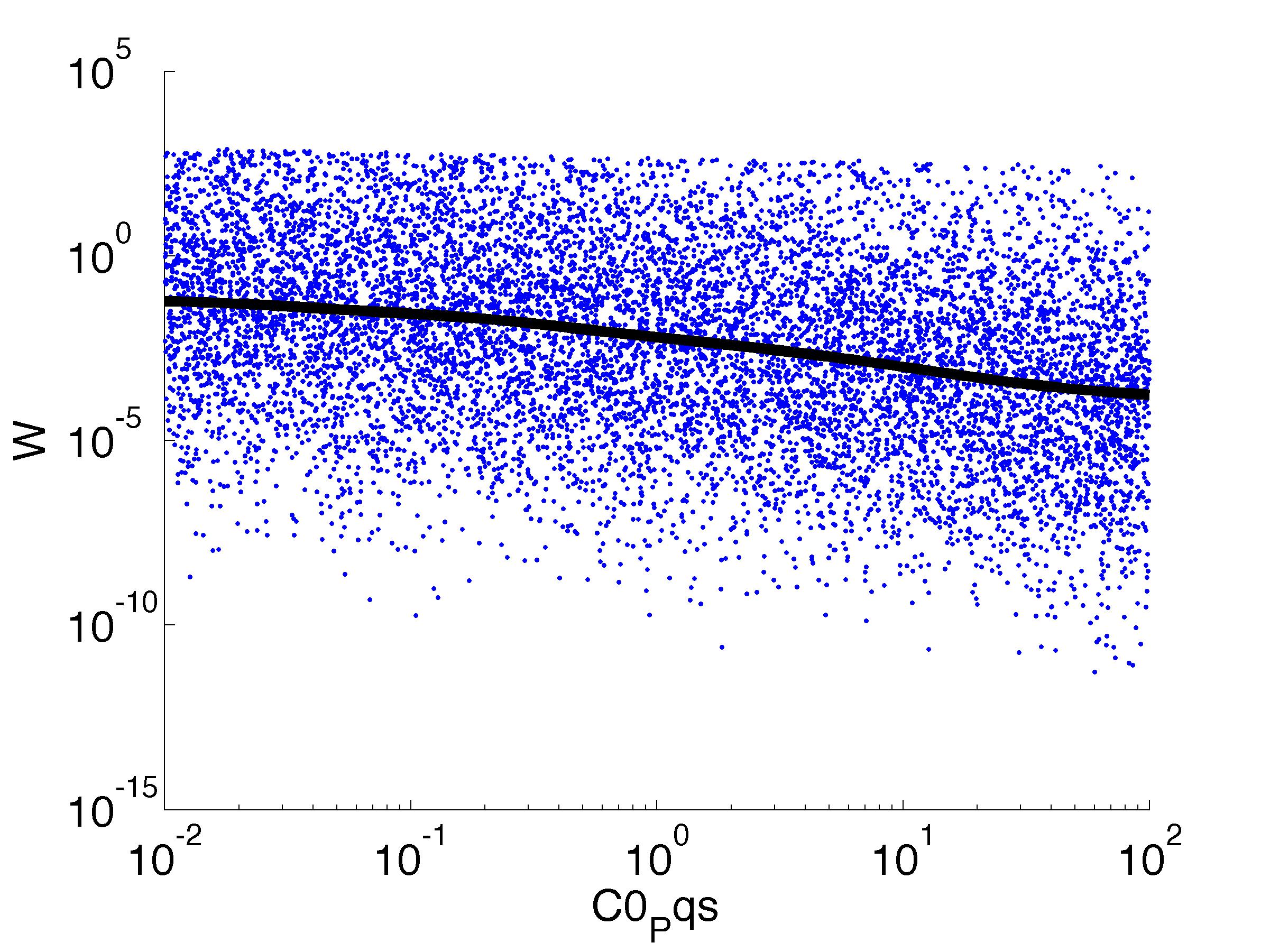
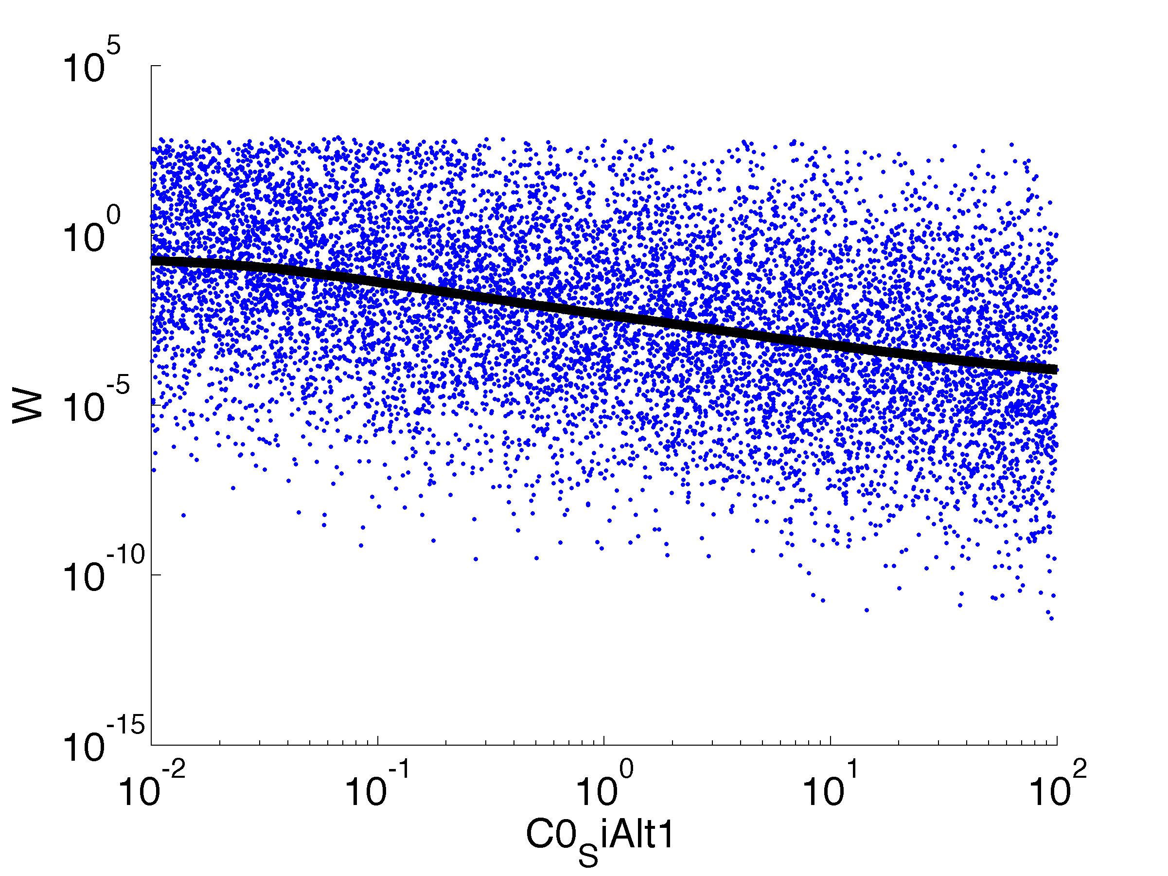
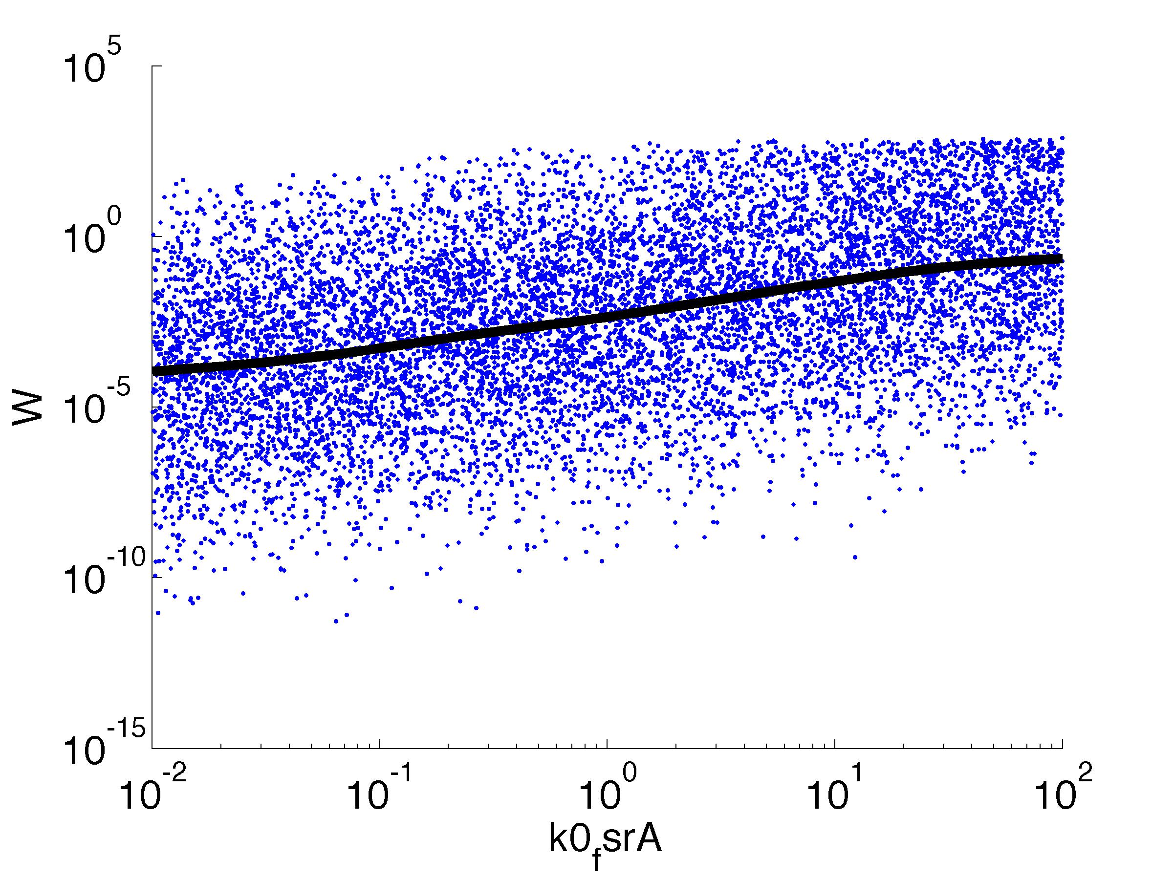
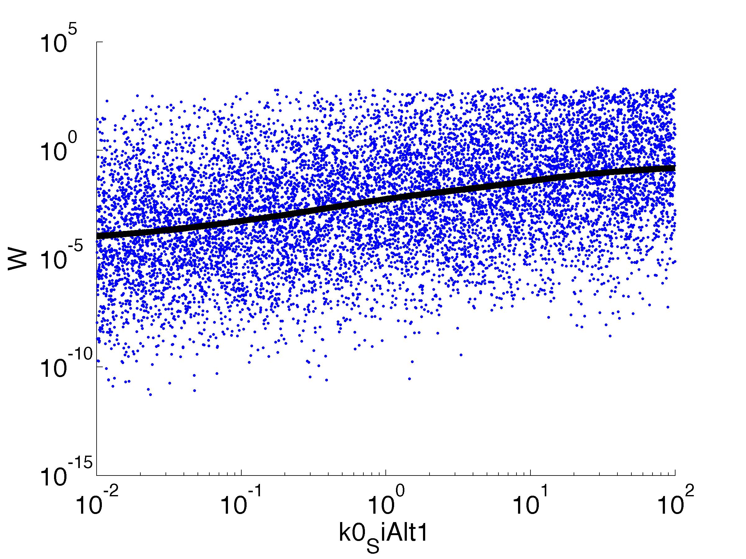
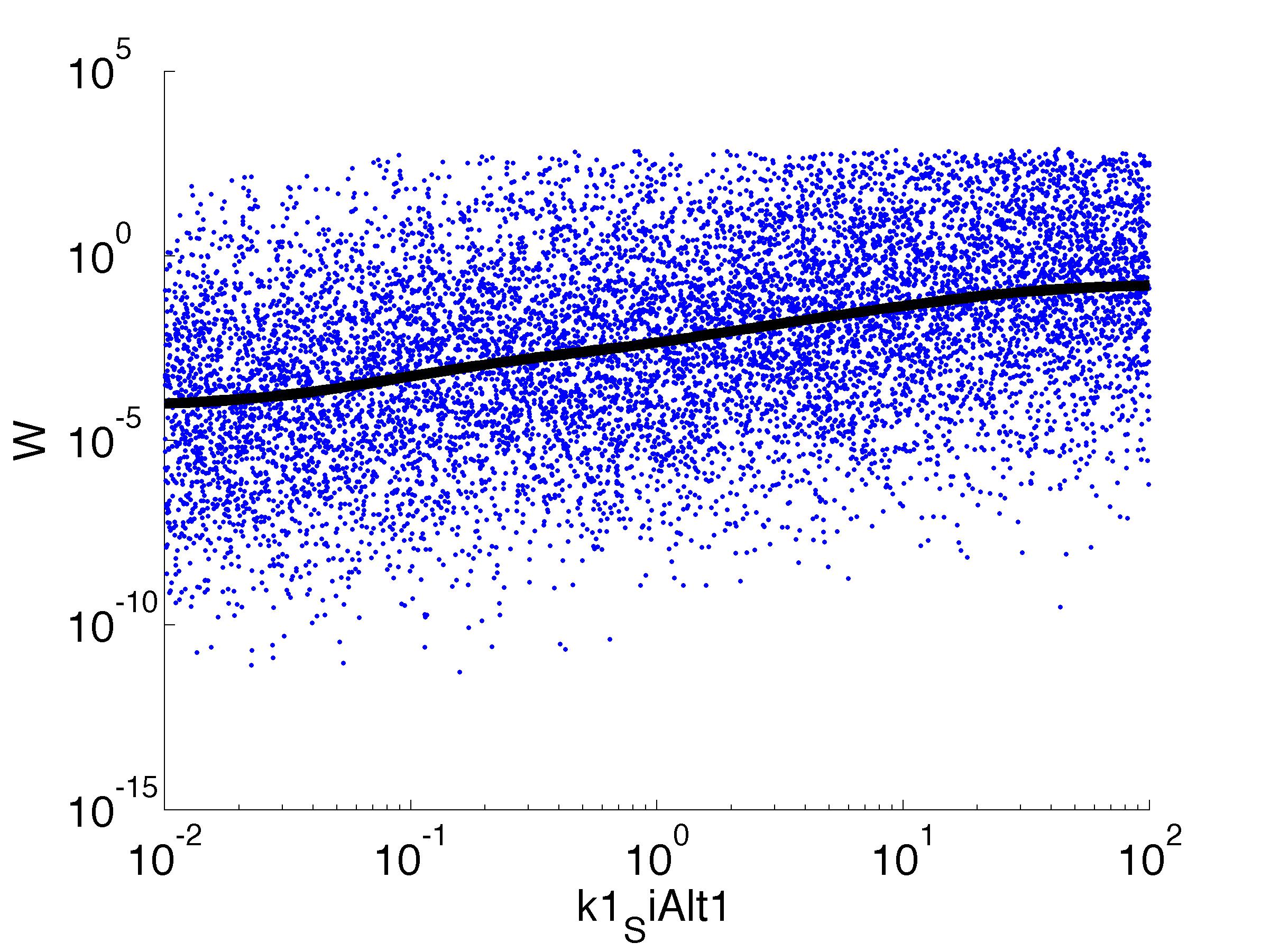
For analysis of the impact of each parameters, we used a function to determine the fitness W of the model. The fitness describes the integral of the surplus of toxic cannibalism proteins over the proprietary antidote. Therefore, a successful suicide equals a high fitness of the model. As we do not know the parameters in for our model we sampled the whole parameter space using a uniform sampler. Successively we used a Nadaraya-Watson kernel densiy estimator to approximate the expected value of W given a single parameter value. This allows us to asses the expected change in W when changing a single parameter, whithout knowledge of all other parameters.
As we can see..... some go up. some go down. one doesn't matter at all. we now know what parameter effect the system in what way.
 "
"

