Team:Oxford/biosensor characterisation

From 2014.igem.org

(Difference between revisions)
(proofread)
Line 481: Line 481:
<img src="https://static.igem.org/mediawiki/2014/4/46/Oxford_data2.png" style="float:right;position:relative; width:80%;margin-left:10%;margin-right:10%;" />
<br><br>
<br><br>
-
We then ran the model for the correct amount of time (2 hours 20mins incubation with ATC) and ran it for lots of different concentrations of ATC over the range that the wet-la team tried. The parameters are still arbitrary at this point (the same as above) but the input values are now correct. This means that the results of these graphs are still arbitrary at this point. The graphic below shows how we used the existing model to obtain the same graphs as the wet-lab team had obtained.
+
We then ran the model for the correct amount of time (2 hours 20mins incubation with ATC) and ran it for lots of different concentrations of ATC over the range that the wet-lab team tried. The parameters are still arbitrary at this point (the same as above) and the results of the graphs are therefore arbitrary are as well, but the input values are now correct. The graphic below shows how we used the existing model to obtain the same graphs as the wet-lab team had obtained.
<br><br>
<br><br>
The numerical inputs that were used to model this data set were therefore:
Line 494: Line 494:
<h1>Parameters</h1>
<h1>Parameters</h1>
-
As all results are arbitrary up to this point, it is now time to calculate the parameters that will make the model’s response match up with the wet-lab data. The purpose of doing this is then the model will be able to give relatively accurate predictions of the response of the bacteria to further testing, therefore making the development of the biosensor much more efficient. The amount of data here will not allow us to calculate the parameters to a high level of accuracy but it should be able to give us some very good approximations of what we can expect.
+
As all results are arbitrary up to this point, it is now time to calculate the parameters that will make the model’s response match up with the wet-lab data. The purpose of doing this is that the model will be able to give relatively accurate predictions of the response of the bacteria to further testing, therefore making the development of the biosensor much more efficient. The amount of data here will not allow us to calculate the parameters to a high level of accuracy, but it should be able to give us some very good approximations of what we can expect.
<br><br>
<br><br>
Line 507: Line 507:
<li>β1 = Basal transcription rate of <font style="font-style: italic;">dcmR</font></li>
-
Remember that because the mCherry gene is tagged (translational fusion) onto the end of the <font style="font-style: italic;">dcmR</font> gene, <font style="font-style: oblique;"> the mCherry fluorescence will be the same as the amount of DcmR protein present</font>. However, there is not very comprehensive data in the literature about the values that we can expect from the behaviour of the <font style="font-style: italic;">dcmR</font> gene.
+
Remember that because the mCherry gene is tagged (translational fusion) onto the end of the <font style="font-style: italic;">dcmR</font> gene, <font style="font-style: oblique;"> the mCherry fluorescence will be the same as the amount of DcmR protein present</font>. However, there is not very comprehensive data in the literature about the values that we can expect from the behaviour of the <font style="font-style: italic;">dcmR</font> gene and its stability in vivo.
<br><br>
<br><br>

Revision as of 10:58, 14 October 2014


Characterisation


Introduction: what are we characterising?

Methylobacterium Extorquens DM4 in the presence of DCM expresses DcmA, a dichloromethane dehalogenase. Within 1.5kb upstream of dcmA and in the opposite orientation is a second gene encoding DcmR, a regulatory protein that controls expression of DcmA:


In order to design and create a stable and sensitive system that responds to DCM we first need to characterise the regulatory nature of DcmR. Characterisation of this regulatory network has never been done before although it has been suggested to be a repressor [1]; we will be the first to fully characterise the mode of action of dcmR. To do this we suppose the following hypotheses for DCM activating the transcription of dcmR: either double repression or double activation. In other words, either DcmR represses dcmA expression and DcmR is in turn repressed by the presence of DCM; or expression of dcmA requires DcmR as an activator, with DcmR in turn only activated in the presence of DCM.

What is currently known about DcmR?

DcmR and regulation of dcmA expression

Mutants with dcmA and the intergenic region but without complete dcmR express DcmA constitutively. Re-integration of dcmR restores regulation of dcmA expression at the transcriptional level [1]. In addition, it has been shown that the region including dcmR, the intergenic region and dcmA is sufficient to confer a DCM dependent response in genetically engineered Methylobacterium extorquens DM4 [2].

DcmR and DNA-binding

DcmR is thought to be a DNA binding protein as structure predicting software indicates that there is a helix-turn-helix domain at the N-terminal of the protein. Since the region between the two promoters for dcmR and dcmA can be deleted without any effect on regulation it has been suggested that DcmR does not to a secondary regulatory site in between the genes but most likely acts directly on the dcmA promoter itself [1]. In addition, regulated expression of dcmA is not effected when the dcmR and dcmA transcriptional units are placed on separate replicons thereby suggesting that their topology is independent of the regulatory network. It is therefore suggested that DcmR binds the DNA in the intergenic region with the simplest model of its mode of action being as a trans-acting DNA-binding repressor; however this remains to be fully validated [1].

We have therefore proceeded on the assumption that DcmR is directly influenced by the presence or absence of DCM and furthermore that we can use dcmR, the intergenic region and dcmA alone to characterise the regulatory network.

[1] La Roche, S. D., and T. Leisinger. "Identification of dcmR, the regulatory gene governing expression of dichloromethane dehalogenase in Methylobacterium sp. strain DM4." Journal of bacteriology 173.21 (1991): 6714-6721.
[2] Lopes, N., et al “Detection of dichloromethane with a bioluminescent (lux) bacterial bioreporter” J Ind Microbiol Biotechnol (2012) 39:45–53

Characterising the DcmR - DCM - P_dcmA interaction

To find out whether the gene dcmR acts as a repressor or an activator on the promoter of the dcmA gene, we attempted to build the genetic circuit shown above on the right. Having dcmR under inducible TetR expression should allow us to have very good control of the amount of DcmR present. On top of this, attaching the mCherry fluorescence tag will act as another confirmation to the amount of DcmR present.

We then extensively modelled the circuit to discover how the response of the system would differ if it was either of the two circuit systems. Click the modelling bubbles (pink) to find out exactly how we achieved this.
Modelling the first half of the genetic circuit

Predicting the mCherry fluorescence

We simplified the first double repression by modelling it as an activation of dcmR by ATC, albeit parameterised by different constants. This assumption is justified by the fact that we are able to precisely control the addition of ATC and measure the fluorescence of the mCherry.

We modelled this first step using both deterministic and stochastic models.

Biochemical equations

The biochemical equations that describe the behaviour of the top half of the genetic circuit are:

Oxford iGEM 2014

Deterministic

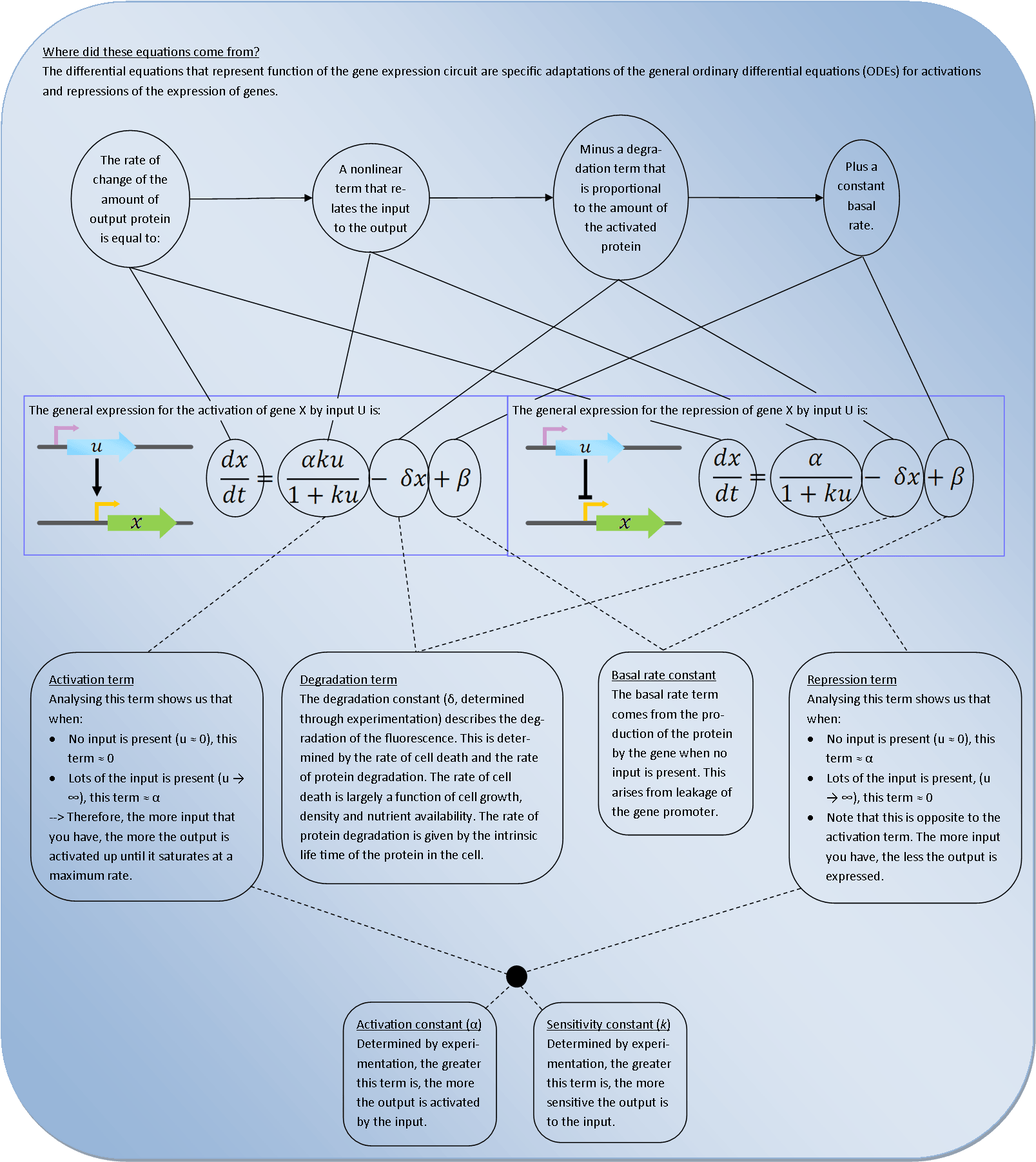
Deterministic models are very powerful tools for synthetic biology. They describe the behaviour of the bacteria at the population level and use Ordinary Differential Equations (ODEs) to relate each activation and repression. By constructing a cascade of differential equations one can build a realistic model of the average behaviour of the system.
The differential equation that descibes this first step of the system is:


Solving this ODE in Matlab

(with zero basal transcription rate)

predicts the following the response of the system:

This model works assuming that

sufficient TetR

is always present.

Oxford iGEM 2014
While the analysis of this circuit is not critical to the successful outcome of this part of the project, it will provide us with very good practice of both obtaining fluorescence time series data and accurately fitting the data to the model. It will also help us develop our methods of predicting future system behaviour. This is because this system is already well documented in the literature and so we should be able to test our methods and responses against well documented results from labs across the world.

As you can clearly see from the graph, the model predicts a large fluorescence increase as the input is added. This is the what we expect from the actual system and is the best approximation that is obtainable before we get experimental data.

In the graph above, the model is set to have a basal transcription rate of zero. This is why there is a zero fluorescence response before the input has been added - this corresponds to the tetO promoter not being leaky at all. This basal rate will be calibrated alongside all of the other parameters in the model.

Stochastic Modelling

Stochastic modelling uses probability theory to predict the behaviour of a system. For our project, we used it to model the expression of GFP from bacteria.

We started with the Gillespie Algorithm, which considers the expression of GFP to be binary; a molecule of GFP is either produced or degraded. We modelled the probability of a molecule of GFP being created using the Michaelis-Menten model, incorporating a basal transcription rate. For the degradation, we assumed a simple proportional relationship; the more you have the more likely it is that a molecule degrades. The constant of proportionality will be a function of the intrinsic life time of the protein in the cell. Now at every increment in time we will not have a GFP reaction occurring, so before we decided what reaction occurs we had to work out if I a reaction occurred. We did this by writing an equation involving the probability of any reaction occurring with a random number generator. To work out which reaction occurred we compared the relative probability of a production to degradation, and used a random number to make a weighted choice.

We later changed this code so that a reaction occurred every time increment, but included a null reaction where no GFP was degraded or created. Although this made the code a lot more data heavy, it allowed for much easier calculation of the mean response of multiple realisations.

Stochastic modelling is useful because it can show us the stochastic effects which are often seen in real bacteria. By calculating the variation of the mean of multiple GFP producing bacteria, we can also work out the standard deviation. Then if we assume that the system varies with respect to the normal distribution, we can produce error bounds for the production of GFP. Such that we can say, 90% of the time we can expect the production of GFP from a single bacterium to be within these 2 curves. This could be useful for seeing if results are unexpected, or, if there are multiple outliers, that our model is incorrect. If we average more and more bacteria then the mean curve tend towards the deterministic response. This is to be expected as we are now looking at the system as a whole and fluctuations in the production from individual bacteria are averaged out. Sto for small Det for large What is stochastic modelling? -- Yes How is it useful? Ads/Dis -- Getting there Tending to deterministic -- Yes Modelling activator repressor --? Parameter characterisation/Data matching -- Not yet Matlab graphs – Not yet Improve Gillespie algorithm bit
  • Matlab graphs
  • How can we tell the systems apart?
    How can we tell the systems apart?

    Predicting the sfGFP fluorescence

    Introduction

    To allow us to characterize the second half of the genetic circuit, we needed to be able to predict the difference in response. To do this, we constructed models by cascading the differential equations according to the respective circuit structures thereby producing two different potential system responses.

    To achieve this, we constructed simplified equivalent circuits that were linked by two potential activation-repression relationships.

    It is important to understand that these simplified equivalent circuits will not give the correct mCherry response but they will give the correct GFP response after correct parameterisation.

    We then set up the differential equations necessary to solve this problem in Matlab. The method and results are as detailed below:

    INSERT SENSITIVITY GRAPH HERE


    Oxford iGEM 2014

    Conclusion

    The bottom graphs illustrate the predicted response of each system to a simultaneous step input of both DCM and ATC. As you can see, there is little difference in the predicted steady-state value of the fluorescence, however, providing the basal transcription rate of GFP is relatively low, there should be a clear difference in the level of fluorescence before either of these inputs are added. This very easily identifiable difference between the two systems will enable us to characterize the genetic circuit present in our particular system.

    Calculating the parameters

    Calculating the many parameters for this system will be undoubtedly challenging.

    How are we calculating the parameters?

    Go to the data section where we calculated parameters for this part of the circuit.
    ATC induction of mCherry expression
    ATC induction of mCherry expression

    Wetlab data showing response in level of mCherry expressed with different concs of ATC

    By making a translational fusion of mCherry at the C terminus of the dcmR gene under the tet promoter and tet operator system(see our Construction page for details) we could measure mCherry fluorescence to gain information about dcmR induction by ATC. Expression was induced with various amounts of ATC and the following fluorescence data acquired. Exposure time was 0.2 seconds. As no calibration data was obtained using purified mCherry, the results have been left in fluorescence arbitrary units. Images were analysed using imageJ software.
    mCherry fluorescence increases with amount of ATC used confirming that the dcmR gene was expressed under the control of the tet promoter and operator system.


    This data was then used to refine and test our models (see below).


    Fitting data and finding parameters
    Fitting data and finding parameters

    Introduction

    As you can see from the biochemistry bubble above, our team was only able to obtain fluorescence data for the first half of the genetic circuit (ATC induced mCherry response). On top of this, the wet lab team were unable to obtain data that measured how the fluorescence of a single culture changed with time, again because of time constraints. This is slightly limiting because it means that we don’t have any dynamic data for any part of our system, and therefore can’t test the modelling predictions of the speed of the biosensor’s response.

    The original data is shown on the right with error bars showing the standard error of the measurements.

    Standard error is calculated as the average standard deviation divided by the square root of the total number of readings.

    How we used the model

    However, to demonstrate the power of the computer models that we’ve built, we made our model simulate the same graph (mean fluorescence against ATC concentration added). To build this, we started from the graph shown in the first modelling bubble on this page, shown here with a small basal rate (see where did these equations come from? ). This graph shows how the predicted fluorescence of the cells changes with time in response to an addition of ATC halfway along the time scale. At this stage, all input values, model parameters and therefore results are arbitrary.


    We then ran the model for the correct amount of time (2 hours 20mins incubation with ATC) and ran it for lots of different concentrations of ATC over the range that the wet-lab team tried. The parameters are still arbitrary at this point (the same as above) and the results of the graphs are therefore arbitrary are as well, but the input values are now correct. The graphic below shows how we used the existing model to obtain the same graphs as the wet-lab team had obtained.

    The numerical inputs that were used to model this data set were therefore:


    Parameters

    As all results are arbitrary up to this point, it is now time to calculate the parameters that will make the model’s response match up with the wet-lab data. The purpose of doing this is that the model will be able to give relatively accurate predictions of the response of the bacteria to further testing, therefore making the development of the biosensor much more efficient. The amount of data here will not allow us to calculate the parameters to a high level of accuracy, but it should be able to give us some very good approximations of what we can expect.


    The parameters that we need to calculate are the constants in the differential equation that governs the behaviour of the first half of the genetic circuit. This half of the system is shown again here to remind the reader which part we are considering.

    These parameters are:

  • α1 = expression rate constant of dcmR
  • k1 = Michaelis - Menten constant of dcmR
  • d1 = degradation constant of dcmR
  • β1 = Basal transcription rate of dcmR
  • Remember that because the mCherry gene is tagged (translational fusion) onto the end of the dcmR gene, the mCherry fluorescence will be the same as the amount of DcmR protein present. However, there is not very comprehensive data in the literature about the values that we can expect from the behaviour of the dcmR gene and its stability in vivo.

    Degradation constant

    The initial steady state of the system (before ATC has been added) is determined by two constants in the model. These constants are the degradation constant of DcmR and the basal transcription rate of the system. Due to the lack of numerical information in the literature on the behaviour of the dcmR gene, the way of calculating these two parameters is by using the single basal rate data point from the wet-lab data (fluorescence value when 0ng of ATC has been added).

    If we assume that the half-life of the dcmR protein is 3 hours [1] (180 minutes), we can calculate the degradation constant for our model. The exponential protein decay is therefore described by:

    Basal transcription rate

    Expression rate constant and Michaelis - Menten constant


    Sensitivity

    An important part of building mathematical models is sensitivity analysis of the results. This can be basically explained as wiggling all of the input values and parameters to see how much variations in each of these values affects the system output. This is especially important for finding parameters to describe the system as it is important to know what level of accuracy the values need to be found to provide a reasonable degree of prediction accuracy.

    On top of this, it is possible to find what range of values the system is especially sensitive to. An example of this analysis is shown with a simple example that is relevant to our system below:

    Stability

    In our Engineering studies we have learnt detailed control theory. Control theory is an interdisciplinary branch of engineering and mathematics that deals with the behavior of dynamical systems with inputs, and how their behavior is modified by feedback. The usual objective of control theory is to control a system so that its output follows a desired control signal, called the reference, which may be a fixed or changing value. This important because many dynamic systems can go unstable if they are given an unsafe set of input values and/or operating conditions.

    However, as there are no feedback loops in this synthetic circuit, control theory analysis of this system isn't necessary.

    Future experiment ideas from an Engineering design perspective

    Reference

    [1] Dr George Wadhams by personal communication (14/10/2014)
    ATC induction of mCherry expression
    ATC induction of mCherry expression

    Wetlab data showing whether it is a repressor or activator

    data and analysis


    Oxford iGEM 2014