"
"
Team:Oxford/biosensor characterisation
From 2014.igem.org
(Difference between revisions)
MatthewBooth (Talk | contribs) |
Olivervince (Talk | contribs) |
||
| Line 256: | Line 256: | ||
<h1>Predicting the sfGFP fluorescence</h1> | <h1>Predicting the sfGFP fluorescence</h1> | ||
<h1>Introduction</h1> | <h1>Introduction</h1> | ||
| - | To allow us to characterize the second half of the genetic circuit, we needed to be able to predict the difference in response. To do this, we constructed models by cascading the differential equations according to the respective circuit structures thereby producing two different potential system responses. | + | To allow us to characterize the second half of the genetic circuit (DcmR regulating sfGFP), we needed to be able to predict the difference in response. To do this, we constructed models by cascading the differential equations according to the respective circuit structures thereby producing two different potential system responses. |
<br><br> | <br><br> | ||
We then set up the differential equations necessary to solve this problem in Matlab. The method and results are as detailed below: | We then set up the differential equations necessary to solve this problem in Matlab. The method and results are as detailed below: | ||
| Line 503: | Line 503: | ||
<h1>Introduction</h1> | <h1>Introduction</h1> | ||
| - | + | Our team were able to obtain good data for both the mCherry response of the system and the overall sfGFP response. This bubble shows how we adapted our model to make the most of the mCherry fluorescence data. | |
<br><br> | <br><br> | ||
The original data is shown on the right with error bars showing the standard error of the measurements. | The original data is shown on the right with error bars showing the standard error of the measurements. | ||
| Line 883: | Line 883: | ||
<br><br> | <br><br> | ||
<h1>Calculating the parameters</h1> | <h1>Calculating the parameters</h1> | ||
| - | To calculate the parameters for behaviour of the second half of the genetic circuit, we used a similar approach to the method we used to find the parameters for the top half of the circuit. This involves taking key bits of the data and analysing the corresponding equation. | + | To calculate the parameters for behaviour of the second half of the genetic circuit (DcmR regulating sfGFP), we used a similar approach to the method we used to find the parameters for the top half of the circuit. This involves taking key bits of the data and analysing the corresponding equation. |
<br><br> | <br><br> | ||
<h1>Degradation rate constant (δ2)</h1> | <h1>Degradation rate constant (δ2)</h1> | ||
| Line 891: | Line 891: | ||
<h1>Basal transcription rate constant (β3)</h1> | <h1>Basal transcription rate constant (β3)</h1> | ||
| - | To find the basal transcription rate constant of the second half of the system, we analysed the data of the fluorescence of just the Pdcma and the sfGFP gene. | + | To find the basal transcription rate constant of the second half of the system (DcmR regulating sfGFP), we analysed the data of the fluorescence of just the Pdcma and the sfGFP gene. |
<br><br> | <br><br> | ||
| - | The data shown on the graphs below shows clearly that the fluorescence stops | + | The data shown on the graphs below shows clearly that the fluorescence stops increasing when the bacteria stop growing in the log phase. This means that we can’t reliably use the data from the stationary phase to provide parameters. We have taken this point to be 500 minutes into the data measurement. |
<br><br> | <br><br> | ||
| Line 907: | Line 907: | ||
<br><br> | <br><br> | ||
<h1>Expression rate constant (α3) and Michaelis - Menten constant (k3)</h1> | <h1>Expression rate constant (α3) and Michaelis - Menten constant (k3)</h1> | ||
| - | Now that we know two of the four parameters for the second half of our synthetic circuit, we needed to calculate the final two parameters to complete our model. To do this, we analysed wet-lab data that showed the system in the presence of DcmR. This now means that the non linear term in our ODE is non zero and the analysis becomes | + | Now that we know two of the four parameters for the second half of our synthetic circuit (DcmR regulating sfGFP), we needed to calculate the final two parameters to complete our model. To do this, we analysed wet-lab data that showed the system in the presence of DcmR. This now means that the non linear term in our ODE is non zero and the analysis becomes |
<br><br> | <br><br> | ||
This data is shown here. Note the difference in the right hand plot reaffirming that DcmR acts as a repressor on PdcmA. | This data is shown here. Note the difference in the right hand plot reaffirming that DcmR acts as a repressor on PdcmA. | ||
Revision as of 03:05, 18 October 2014


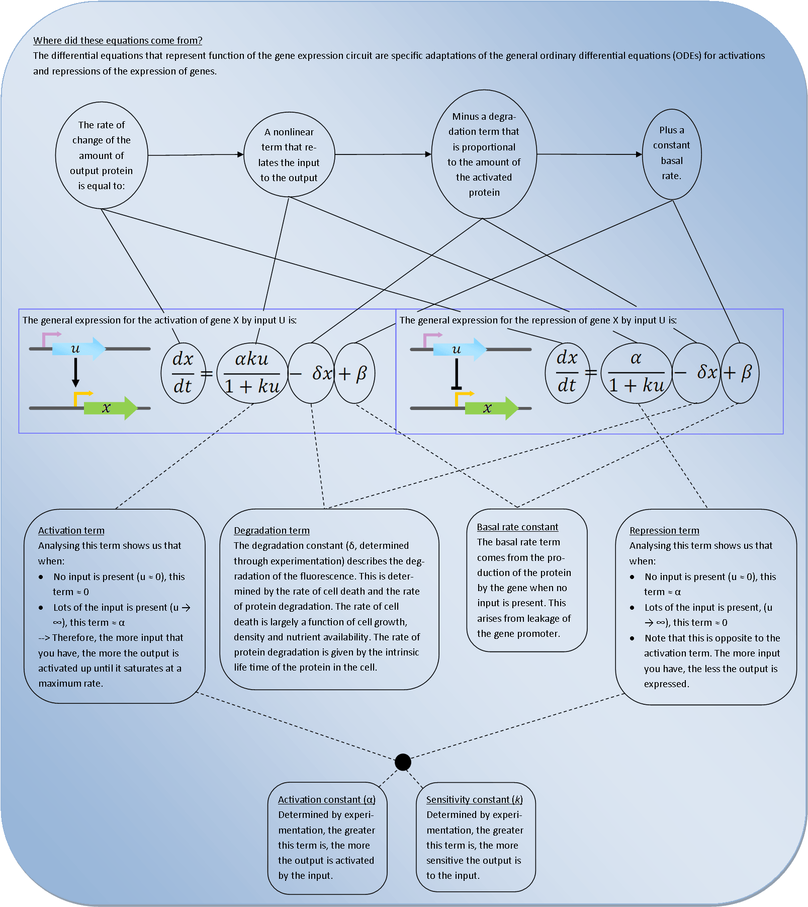
 Deterministic models are very powerful tools for synthetic biology. They describe the behaviour of the bacteria at the population level and use Ordinary Differential Equations (ODEs) to relate each activation and repression. By constructing a cascade of differential equations one can build a realistic model of the average behaviour of the system.


 Oxford iGEM 2014


 This simplifies the equation to:
 As we want our model to accurately predict the fluorescence, we will substitute the fluorescence value in place of the [DcmR] and rearrange:
 Substituting in the value for δ1 that we found above and the basal steady state fluorescence level from the data (471 to 3 s.f.) gives the basal transcription rate as:

 alongside the correct inputs:
 The graph below shows the model's predictions plotted in the same figure as the data points that the wet-lab team obtained for the system:
 Plotting the model's output as a by interpolating between the calculated values makes the graph clearer:


 The results clearly show a decrease in sfGFP fluorescence upon addition and expression of dcmR. Therefore we can confidently conclude that DcmR acts as a repressor in both directions for the PdcmA and PdcmR promoter.

 For the PdcmR promoter both with and without DcmR:
 From these results we can see that in the direction of PdcmA DCM has a modulating effect of relieving DcmR repression thus DCM acts through depression. Interestingly, DCM appears to decrease sfGFP fluorescence in the absence of DcmR.
In the direction of PdcmR DCM appears to have no significant effect on the expression of sfGFP. Therefore in the native system we suggest that DCM has a modulating effect through depression of dcmA expression. Additionally DCM shows no effect on the auto regulation of dcmR expression.
From these results we can see that in the direction of PdcmA DCM has a modulating effect of relieving DcmR repression thus DCM acts through depression. Interestingly, DCM appears to decrease sfGFP fluorescence in the absence of DcmR.
In the direction of PdcmR DCM appears to have no significant effect on the expression of sfGFP. Therefore in the native system we suggest that DCM has a modulating effect through depression of dcmA expression. Additionally DCM shows no effect on the auto regulation of dcmR expression.


 In terms of the modelling equations, this system is equivalent to setting [DcmR] to zero and ensuring that for this scenario, we set β1 = 0 (basal transcription rate of DcmR) . The mathematics below shows how we used the normalised data to find the basal transcription rate of sfGFP. Note how we’re using equation with parameters α3, β3 and k3 because the wet-lab team were able to prove that DcmR acts as a repressor on PdcmA.
 Using the analytical solution outlined above, we were then able to characterize the single unknown parameter in the system (β3 - the basal rate of transcription of sfGFP). By again utilizing our data fitting algorithm alongside our hypothetical value for the basal rate of transcription of sfGFP, β3 was calculated to be 4.6.
 Similar parameter calculation from this data gives:
 More on the further use of this model is available in the