Introduction
As you can see from the biochemistry bubble above, our team was only able to obtain fluorescence data for the first half of the genetic circuit (ATC induced mCherry response). On top of this, the wet lab team were unable to obtain data that measured how the fluorescence of a single culture changed with time, again because of time constraints. This is slightly limiting because it means that we don’t have any dynamic data for any part of our system, and therefore can’t test the modelling predictions of the speed of the biosensor’s response.
The original data is shown on the right with error bars showing the standard error of the measurements.
Standard error is calculated as the average standard deviation divided by the square root of the total number of readings.
How we used the model
However, to demonstrate the power of the computer models that we’ve built, we made our model simulate the same graph (mean fluorescence against ATC concentration added). To build this, we started from the graph shown in the
first modelling bubble
on this page, shown here with a small basal rate (see
where did these equations come from?
). This graph shows how the predicted fluorescence of the cells changes with time in response to an addition of ATC halfway along the time scale. At this stage, all input values, model parameters and therefore results are arbitrary.

We then ran the model for the correct amount of time (2 hours 20mins incubation with ATC) and ran it for lots of different concentrations of ATC over the range that the wet-la team tried. The parameters are still arbitrary at this point (the same as above) but the input values are now correct. This means that the results of these graphs are still arbitrary at this point. The graphic below shows how we used the existing model to obtain the same graphs as the wet-lab team had obtained.
The numerical inputs that were used to model this data set were therefore:

Parameters
As all results are arbitrary up to this point, it is now time to calculate the parameters that will make the model’s response match up with the wet-lab data. The purpose of doing this is then the model will be able to give relatively accurate predictions of the response of the bacteria to further testing, therefore making the development of the biosensor much more efficient. The amount of data here will not allow us to calculate the parameters to a high level of accuracy but it should be able to give us some very good approximations of what we can expect.

The parameters that we need to calculate are the constants in the differential equation that governs the behaviour of the first half of the genetic circuit. This half of the system is shown again here to remind the reader which part we are considering.
These parameters are:
α1 = expression rate constant of dcmR
k1 = Michaelis - Menten constant of dcmR
d1 = degradation constant of mCherry
β1 = Basal transcription rate of dcmR
Remember that because the mCherry gene is tagged onto the end of the
dcmR gene, therefore
the mCherry fluorescence will be the same as the DcmR production from the
dcmR gene. Due to the translational fusion of the mCherry gene onto the
dcmR gene, we can assume that the mCherry protein (and therefore the fluorescence) will degrade with the same rate as the DcmR protein. However, there is not very comprehensive data in the literature about the values that we can expect from the behaviour of the
dcmR gene.
Degradation constant and the basal transcription rate
The initial steady state of the system (before ATC has been added) is determined by two constants in the model. These constants are the degradation constant of DcmR and the basal transcription rate of the system. Due to the lack of numerical information in the literature on the behaviour of the
dcmR gene, the only way of calculating these two parameters is by using the single basal rate data point from the wet-lab data (fluorescence value when 0ng of ATC has been added). Therefore, we have one equation and two unknowns which is bad. To obtain a degree of legitimacy with the values of these two parameters, we decided to use the degradation rate
To calculate the degradation rate constant of the mCherry protein, we turned to the literature as this is a well documented area of synthetic biology. The graph on the above right shows how the fluorescence of the protein decays with time and data in the source document identifies the half-life as 96 seconds.
This graph was sourced from
here.
In terms of the ODE describing the mCherry fluorescence, this graph corresponds to setting the [ATC] value and the basal transcriptional rate to zero, thus leaving the equation below:

From here, simple calculation using this literature data allowed us to calculate that:
d1 = degradation constant of mCherry = 0.416 (mins^-1)
From here, we could then calculate the basal transcription rate...
Sensitivity
An important part of building mathematical models is sensitivity analysis of the results. This can be basically explained as wiggling all of the input values and parameters to see how much variations in each of these values affects the system output. This is especially important for finding parameters to describe the system as it is important to know what level of accuracy the values need to be found to provide a reasonable degree of prediction accuracy.
On top of this, it is possible to find what range of values the system is especially sensitive to. An example of this analysis is shown with a simple example that is relevant to our system below:
Stability
In our Engineering studies we have learnt detailed control theory. Control theory is an interdisciplinary branch of engineering and mathematics that deals with the behavior of dynamical systems with inputs, and how their behavior is modified by feedback. The usual objective of control theory is to control a system so that its output follows a desired control signal, called the reference, which may be a fixed or changing value. This important because many dynamic systems can go unstable if they are given an unsafe set of input values and/or operating conditions.
However, as there are no feedback loops in this synthetic circuit, control theory analysis of this system isn't necessary.
Future experiment ideas from an Engineering design perspective
 "
"


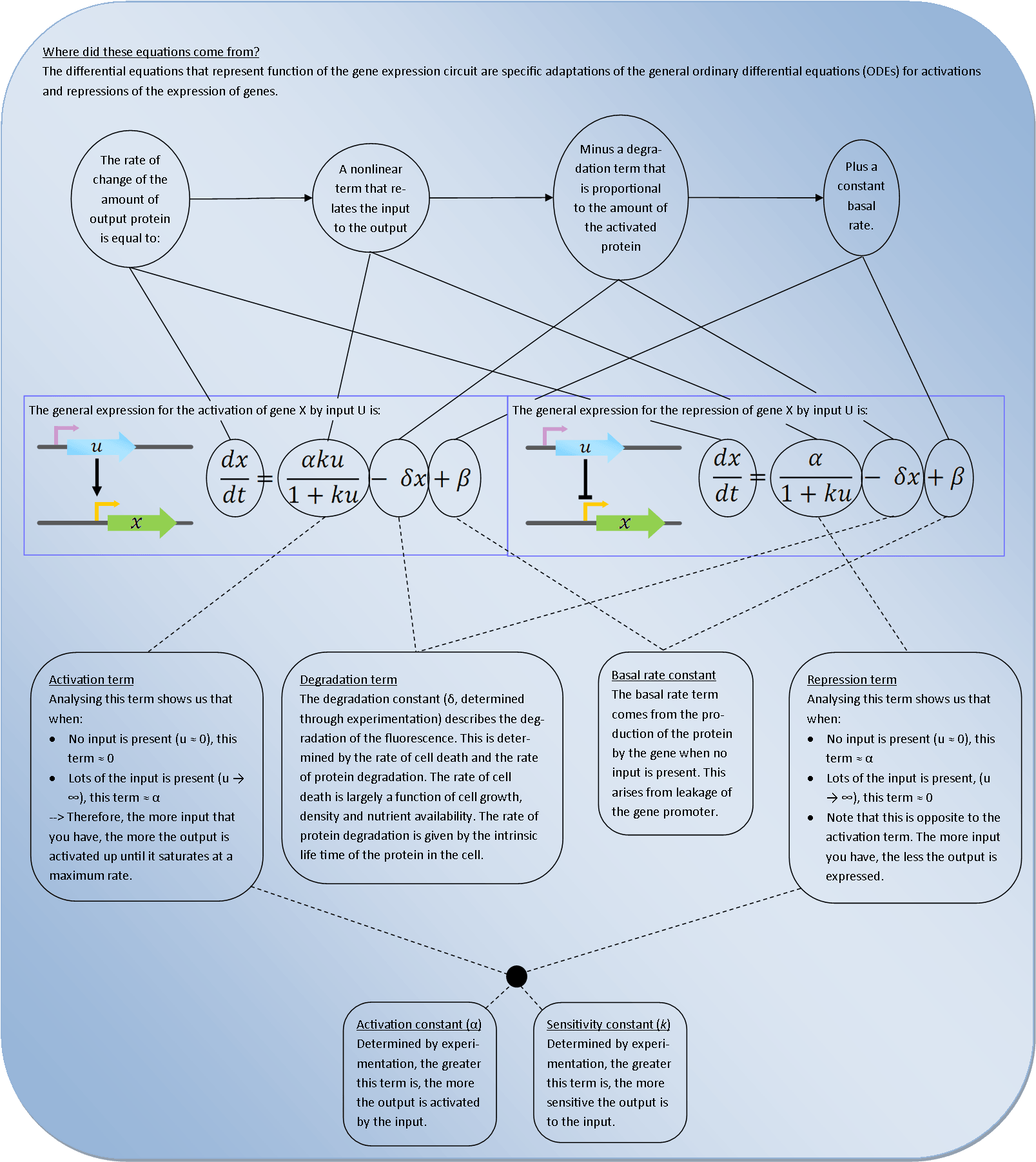
 Deterministic models are very powerful tools for synthetic biology. They describe the behaviour of the bacteria at the population level and use Ordinary Differential Equations (ODEs) to relate each activation and repression. By constructing a cascade of differential equations one can build a realistic model of the average behaviour of the system.


 Oxford iGEM 2014