Team:Valencia UPV/Modeling/diffusion

Since pheromones are chemicals released into the air, we have to consider both the motion of the fluid and the one of the particles suspended in the fluid.

The motion of fluids can be described by the Navier–Stokes equations. But the typical nonlinearity of these equations when there may exist turbulences in the air flow, makes most problems difficult or impossible to solve. Thus, attending to the particles suspended in the fluid, a simpler effective option for pheromone dispersion modeling consists in the assumption of pheromones diffusive-like behavior. That is, pheromones are molecules that can undergo a diffusion process in which the random movement of gas molecules transport the chemical away from its source [1].

There are two ways to introduce the notion of diffusion: either using a phenomenological approach starting with Fick's laws of diffusion and their mathematical consequences, or a physical and atomistic one, by considering the random walk of the diffusing particles [2].

In our case, we decided to model our diffusion process using the Fick's laws. Thus, it is postulated that the flux goes from regions of high concentration to regions of low concentration, with a magnitude that is proportional to the concentration gradient. However, diffusion processes are complex, and modelling them analytically and with accuracy is difficult. Even more when the geometry is not simple (e.g. consider the potential final distribution of our plants in the crop field). For this reason, we decided to consider a simplified model in which pheromone chemicals obey the heat diffusion equation.

Approximation

The diffusion equation is a partial differential equation that describes density dynamics in a material undergoing diffusion. It is also used to describe processes exhibiting diffusive-like behavior, like in our case. The equation is usually written as:

$$\frac{\partial \phi (r,t) }{\partial t} = \nabla · [D(\phi,r) \nabla \phi(r,t)]$$

where $\phi(r, t)$ is the density of the diffusing material at location r and time t, and $D(\phi, r)$ is the collective diffusion coefficient for density $\phi$ at location $r$; and $\nabla$ represents the vector differential operator.

If the diffusion coefficient does not depend on the density then the equation is linear and $D$ is constant. Thus, the equation reduces to the linear differential equation: $$\frac{\partial \phi (r,t) }{\partial t} = D \nabla^2 \phi(r,t)$$

also called the heat equation. Making use of this equation we can write the pheromones chemicals diffusion equation with no wind effect consideration as:

$$\frac{\partial c }{\partial t} = D \nabla^2 C = D \Delta c$$

where c is the pheromone concentration, $\Delta$ is the Laplacian operator, and $D$ is the pheromone diffusion constant in the air.

If we consider the wind, we face a diffusion system with drift, and an advection term is added to the equation above.

$$\frac{\partial c }{\partial t} = D \nabla^2 c - \nabla \cdot (\vec{v} c )$$

where $\vec{v}$ is the average velocity. Thus, $\vec{v}$ would be the velocity of the air flow in or case.

For simplicity, we are not going to consider the third dimension. In $2D$ the equation would be:

$$\frac{\partial c }{\partial t} = D \left(\frac{\partial^2 c }{\partial^2 x} + \frac{\partial^2 c }{\partial^2 y}\right) – \left(v_{x} \cdot \frac{\partial c }{\partial x} + v_{y} \cdot \frac{\partial c }{\partial y} \right) = D \left( c_{xx} + c_{yy}\right) - \left(v_{x} \cdot c_{x} + v_{y} \cdot c_{y}\right) $$

In order to determine a numeric solution for this partial differential equation, the so-called finite difference methods are used. With finite difference methods, partial differential equations are replaced by its approximations as finite differences, resulting in a system of algebraic equations. This is solved at each node $(x_i,y_j,t_k)$. These discrete values describe the temporal and spatial distribution of the particles diffusing.

Although implicit methods are unconditionally stable, so time steps could be larger and make the calculus process faster, the tool we have used to solve our heat equation is the Euler explicit method, for it is the simplest option to approximate spatial derivatives.

The equation gives the new value of the pheromone level in a given node in terms of initial values at that node and its immediate neighbors. Since all these values are known, the process is called explicit.

$$c(t_{k+1}) = c(t_k) + dt \cdot c'(t_k),$$

Now, applying this method for the first case (with no wind consideration) we followed the next steps:

1. Split time $t$ into $n$ slices of equal length dt: $$ \left\{ \begin{array}{c} t_0 &=& 0 \\ t_k &=& k \cdot dt \\ t_n &=& t \end{array} \right. $$

2. Considering the backward difference for the Euler explicit method, the expression that gives the current pheromone level each time step is:

$$c (x, y, t) \approx c (x, y, t - dt ) + dt \cdot c'(x, y, t)$$

3. And now considering the spatial dimension, central differences is applied to the Laplace operator $\Delta$, and backward differences are applied to the vector differential operator $\nabla$ ( in 2D and assuming equal steps in x and y directions):

$$c (x, y, t) \approx c (x, y, t - dt ) + dt \left( D \cdot \nabla^2 c (x, y, t) - \nabla \vec{v} c (x, y, t) \right)$$ $$ D \cdot \nabla^2 c (x, y, t) = D \left( c_{xx} + c_{yy}\right) = D \frac{c_{i,j-1} + c_{i,j+1} + c_{i-1,j } + c_{i+1,j} – 4 c_{I,j}}{s} $$ $$ \nabla \vec{v} c (x, y, t) = v_{x} \cdot c_{x} + v_{y} \cdot c_{y} = v_{x} \frac{c_{i,j} – c_{i-1,j}}{h} + v_{y} \frac{c_{i,j} – c_{i,j-1}}{h} $$

With respect to the boundary conditions, they are null since we are considering an open space. Attending to the implementation and simulation of this method, dt must be small enough to avoid instability.

The Idea

When one stares at moths, they apparently move with erratic flight paths. It is possibly because of predator avoiding reasons.

In this frame, sex pheromones influence in moth behavior is also considered. Since these are pheromones released by females in order to attract an individual of the opposite sex, it makes sense that males respond to gradients of sex pheromone concentration, being attracted towards the source. As soon as a flying male randomly comes into conical pheromone-effective sphere of sex pheromone released by a virgin female, the male begins to seek the females in a zigzag way, approaches to the females and finally copulates with her [1].

Approximation

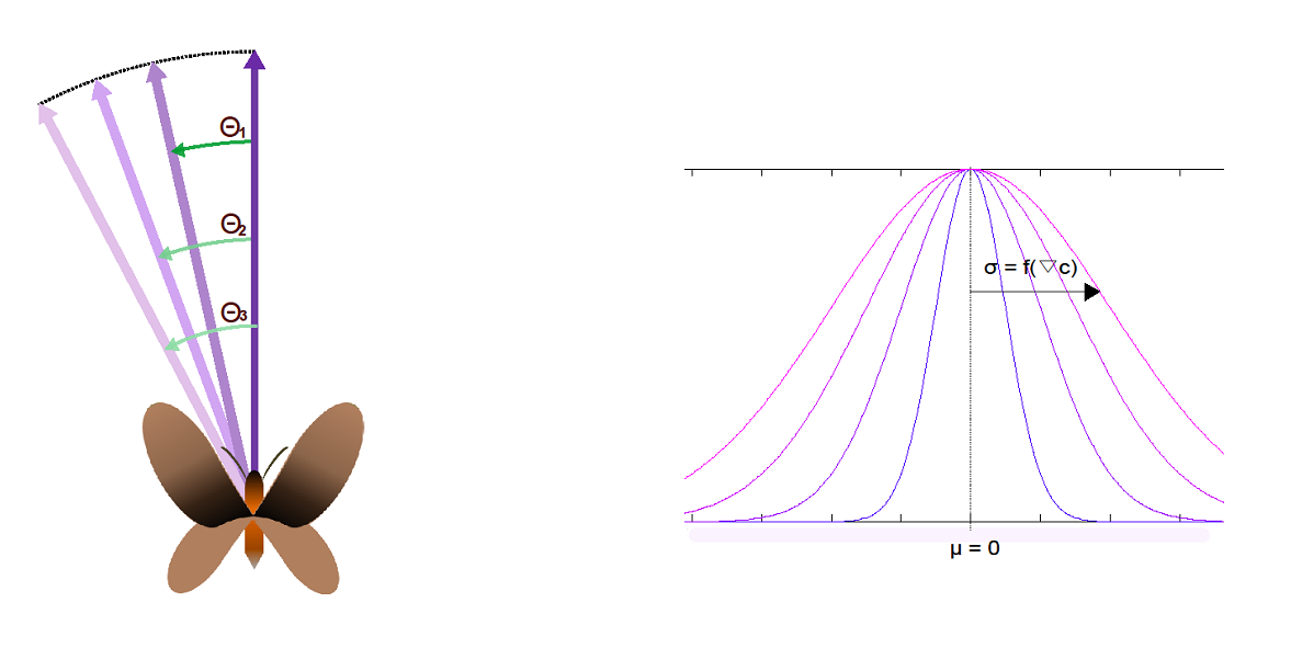
In this project we approximate the resulting moth movement as a vectorial combination of a gradient vector and a random vector. The magnitude of the gradient vector comes from the change in pheromone concentration level among points separated by a differential stretch in space. More precisely, the gradient points in the direction of the greatest rate of increase of the function and its magnitude is the slope of the graph in that direction. The random vector is restricted in this ‘moth response’ model by a fixed angle, assuming that the turning movement is relatively continuous and for example the moth can’t turn 180 relative degrees at the next instant.

Since the objective of this project consists in avoiding pest damage by reaching the mating disrupting among moths, our synthetic plants are supposed to release enough sexual pheromone so as to saturate moth perception. In this sense the resulting moth vector movement will depend ultimately on the pheromone concentration levels in the field and the moth ability to follow better or worse the gradient of sex pheromone concentration.

At this point, let’s highlight the three main aspects we consider for the characterization of males moth behavior:

In this context, this ensemble of behaviors could be translated in a sum of vectors in which the random vector has a constant module and changeable direction inside a range, whereas the gradient vector module is a function of the gradient in the field. The question now is: how do we include the saturation effect in the resulting moth shift vector?

With this in mind and focusing on the implementation process, our approach consists on the following:

The gradient vector instead of experiencing a change in its magnitude, this will be always the unit and its direction that of the greatest rate of increase of the pheromone concentration. A random direction vector with constant module will not be literally considered, but a random turning angle starting from the gradient vector direction.

Attending to the previous question how do we include the saturation effect in the resulting moth shift vector?, here the answer: the dependence on the moth saturation level (interrelated with the pheromone concentration in the field) will state in the random turning angle.

This random turning angle will not follow a uniform distribution, but a Poisson distribution in which the mean is zero (no angle detour from the gradient vector direction) and the standard-deviation will be inversely proportional to the intensity of the gradient of sex pheromone concentration in the field. This approach will drive to a ‘sexual confusion’ of the insect as the field homogeneity increases, since the moth in its direction of displacement will fit the gradient direction with certain probabilities which depend on how saturated they are.

References:

1. Yoshitoshi Hirooka and Masana Suwanai. Role of Insect Sex Pheromone in Mating Behavior I. Theoretical Consideration on Release and Diffusion of Sex Pheromone in the Air.
2. W. L. Roelofs and R. T. Carde. Responses of Lepidoptera to Synthetic Sex Pheromone Chemicals and their Analogues.

Using a modeling environment called Netlogo, we try to simulate the approximate moth population behavior when pheromone diffusion processes are given.

Netlogo simulator can be find in its website at Northwestern University.

To download the source file of our Sexyplant simlation in Netlogo click here: sexyplants.nlogo

SETUP:

• We consider three agents: male and female moths, and sexyplants.
• We have two kind of sexual pheromone emission sources: female moths and sexyplants.
• Our scenario is an opened crop field where sexyplants are intercropped and moths fly following different patterns depending on its sex.

Females, apart from emitting sexual pheromones, they move with erratic random flight paths. After mating, females are 2 hours in which they are not emitting pheromone.

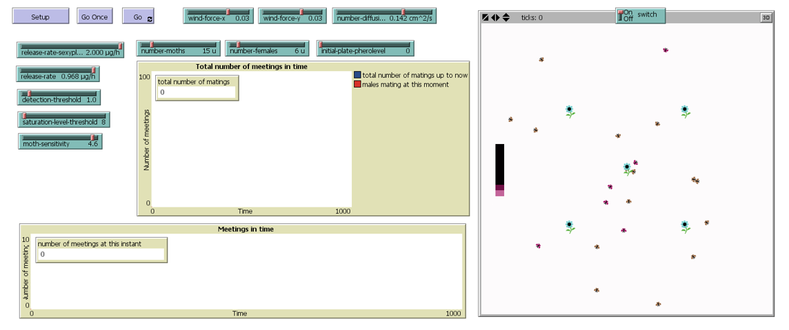
Males also move randomly while they are under its detection threshold. But when they detect a certain pheromone concentration, they start to follow the pheromone concentration gradients until its saturation threshold is reached.

sexyplants act as continuously- emitting sources and their activity is regulated by a Switch.

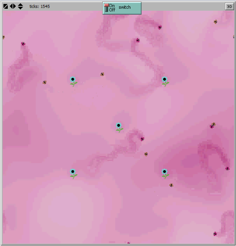
On the side of pheromone diffusion process, it is simulated in Netlogo by implementing the Euler explicit method.

GO!

When sexyplants are switched-off, males move randomly until they detect pheromone traces from females, in that case they follow them.

When sexyplants are switched-on, the pheromone starts to diffuse from them, rising up the concentration levels in the field. At first, the sexyplants have an effect of pheromone traps on the male moths.

As the concentration rises in the field, it becomes more homogeneous. Remember that the random turning angle of the insect follows a Poisson distribution, in which the standard-deviation is inversely proportional to the intensity of the gradient. Thus, the probability of the insect to take a bigger detour from the faced gradient vector direction is higher. This means that it is less able to follow pheromone concentration gradients, so ‘sexual confusion’ is induced.

Parameters

The parameters of this model are not as well-characterized as we expected at first. Finding the accurate values of these parameters is not a trivial task, in the literature it is difficult to find a number experimentally obtained.

So we decided to take an inverse engineering approach. Doing a model parameters swept, we simulate many possible scenarios, and then we come up with values of parameters corresponding to our desired one: insects get confused. This will be useful to know the limitations of our system and to help to decide the final distribution of our plants in the crop field.

Diffusion coefficient

Range of search: 0.01-0.2 cm^2/s
References: [1], [2], [3], [5]

Release rate (female)

Range of search: 0.02-1 µg/h
References: [4], [5]

Release rate (sexyplant)

The range of search that we have considered is a little wider than the one for the release rate of females.
References: It generally has been found that pheromone dispensers releasing the chemicals above a certain emission rate will catch fewer males. The optimum release rate or dispenser load for trap catch varies greatly among species [4]. This certain emission rate above which male start to get confused could be the release rate from females.

Detection threshold

Range of search: 0.001-1 [Mass]/[Distante]^2

Saturation threshold

Range of search: 1-5[Mass]/[ Distante]^2

Moth sensitivity

This is a parameter referred to the capability of the insect to detect changes in pheromone concentration in the patch it is located and the neighbor patch. When the field becomes more homogeneous, an insect with higher sensitivity will be more able to follow the gradients.
Range: 0-0.0009
(The maximum level of moth sensitivity has to be less than the minimum level of release rate of females, since this parameter is obtained from the difference)

Wind force

Range: -0.1 – 0.1 cm/sec
References: [7] (700cm/sec!!!)

Population

The number of males and females can be selected by the observer.

Ticks (time step) !!!

We’ll consider the equivalence 20 ticks= 1 hour. That is 1 tick = 3 minutes.

Patches !!!

The approximate velocity of a male moth flying towards the female in natural environment is 0.3 m/sec [6]. Each moth moves 1 patch per tick, so if 1 tick is equal to 3 minutes (180 sec), the patch is 54 meter long to get that velocity.

One can modify the number of patches that conform the field so as to analyze its own case.

References:

1. Wilson et al.1969, Hirooka and Suwanai, 1976.
2. Monchich abd Mauson, 1961, Lugs, 1968.
3. G. A. Lugg. Diffusion Coefficients of Some Organic and Other Vapors in Air.
4. W. L. Roelofs and R. T. Carde. Responses of Lepidoptera to Synthetic Sex Pheromone Chemicals and their Analogues, Page 386.
5. R.W. Mankiny, K.W. Vick, M.S. Mayer, J.A. Coeffelt and P.S. Callahan (1980) Models For Dispersal Of Vapors in Open and Confined Spaces: Applications to Sex Pheromone Trapping in a Warehouse, Page 932, 940.
6. Tal Hadad, Ally Harari, Alex Liberzon, Roi Gurka (2013) On the correlation of moth flight to characteristics of a turbulent plume.
7. Average Weather For Valencia, Manises, Costa del Azahar, Spain.

The aim consists of reducing the possibility of meeting among moths of opposite sex. Thus, we will analyze the number of meetings in the three following cases:

1. When sexyplants are switched-off and males only interact with females.
2. When sexyplants are switched-on and have an effect of trapping males.
3. When sexyplants are swiched-on and males get confused when the concentration of pheromone level is higher than their saturation threshold.

It is also interesting to analyze a fourth case, what does it happen if females wouldn’t emit pheromones and males just move randomly through the field? :

4. Males and females move randomly. How much would our results differ from the rest of cases?

What is important is that between the first and the third case, the number of meetings should be less in the latter than in the former. Then we are closer to our objective fulfillment.

References

- Sol I. Rubinow, Mathematical Problems in the Biological Sciences, chap. 9, SIAM, 1973
- J. N. Perry and C. Wall , A Mathematical Model for the Flight of Pea Moth to Pheromone Traps Through a Crop, Phil. Trans. R. Soc. Lond. B 10 May 1984 vol. 306 no. 1125 19-48
- J. Philibert. One and a half century of diffusion: Fick, Einstein, before and beyond. Diffusion Fundamentals, 2,1.1-1.10, 2005.