Team:NCTU Formosa/modeling

From 2014.igem.org

Revision as of 20:43, 17 October 2014 by Roy (Talk | contribs)

Modeling

Change the font size right here

Contents

Modeling Introduction

In the modeling part, we make two models in our project to optimize our result and enhance the convenience of the device usage. In the first model, we demonstrate a model for our biobricks which is composed of Pcons, RBS, 9 PBAN, BFP, and Terminator. And in the second model, we model our device with two kinds of natural factor which are temperature and the wavelength of light.

In this project, we use two main function of ANFIS, which is data adjusting and data simulating, in our PBAN model and device model. In PBAN model, we use a theoretical biobrick to adjust our experiment data, and in device model, we use the simulation function to find a prediction surface to predict the insect capture performance of our device. These result will describe in the following parts.

The following contents we can divide into three parts:

(1) Modeling of PBAN: First, we use ANFIS to build PBAN model that can fit to theoretical estimation and real condition at the    same time.

(2) Modeling of Device: Second, a device model is also established. This model can let the user know the insect capture       performance in any condition.

(3) Modeling Software: At last, we introduce the tool we use. ANFIS, a tool involved in MATLAB.

Modeling of PBAN

In this project, 9 kinds of PBAN are used to attract 9 different kinds of insects into our device. Even though these 9 PBAN (PBAN(BM), PBAN(MB), PBAN(AI), PBAN(LD), PBAN(HAH), PBAN(AS), PBAN(SI), PBAN(AA), PBAN(SL)) facilitates the production of pheromone through different pathways, 9 PBAN are translated with the same promoter and RBS in E. coli, and therefore, the production rate for each PBAN should be the same. With that said, we use a “Pcons + RBS + BFP + Ter” as the theoretical condition to simulate PBAN biobrick (Pcons + RBS + PBAN + BFP + Ter) expression. By detecting the expression value from the theoretical biobrick and modifying by our PBAN biobrick expression, this modified model can not only fit a theoretical condition that prevents our model from operating bias, but also fit to a real condition. To make a brief introduction of our PBAN model, the following contents are divided into two parts: (1) Theoretical biobrick (2) 9 different kinds of PBAN biobrick and modeling result.

Theoretical biobrick
Fig.2-1-1 A biobrick used as a template to simulate the PBAN biobrick expression.
Fig.2-1-2 Theoretical biobrick expression profile.
9 different kinds of PBAN biobrick and modeling result
1. Pcons + RBS + PBAN(BM) + BFP + Ter
Fig.2-2-1 Biobrick of Pcons + RBS + PBAN(BM) + BFP + Ter.
Fig.2-2-2 Modeling result of Pcons + RBS + PBAN(BM) + BFP + Ter. The blue line is the expression profile of the theoretical biobrick. And the green line is the expression data of Pcons + RBS + PBAN(BM) + BFP + Ter. And the red line is the adjusting line from the green and blue one. This line represent the correcting line of theoretical data and real condition data which can make our model not only fit the theoretical condition but also stay away from experimental bias.


2. Pcons + RBS + PBAN(MB) + BFP + Ter
Fig.2-2-3 Biobrick of Pcons + RBS + PBAN(MB) + BFP + Ter.
Fig.2-2-3 Modeling result of Pcons + RBS + PBAN(MB) + BFP + Ter. The blue line is the expression profile of the theoretical biobrick. And the green line is the expression data of Pcons + RBS + PBAN(MB) + BFP + Ter. And the red line is the adjusting line from the green and blue one. This line represent the correcting line of theoretical data and real condition data which can make our model not only fit the theoretical condition but also stay away from experimental bias.


3. Pcons + RBS + PBAN(SL) + BFP + Ter
Fig.2-2-6 Biobrick of Pcons + RBS + PBAN(SL) + BFP + Ter.
Fig.2-2-7 Modeling result of Pcons + RBS + PBAN(SL) + BFP + Ter. The blue line is the expression profile of the theoretical biobrick. And the green line is the expression data of Pcons + RBS + PBAN(SL) + BFP + Ter. And the red line is the adjusting line from the green and blue one. This line represent the correcting line of theoretical data and real condition data which can make our model not only fit the theoretical condition but also stay away from experimental bias.


4. Pcons + RBS + PBAN(AI) + BFP + Ter
Fig.2-2-8 Biobrick of Pcons + RBS + PBAN(AI) + BFP + Ter.
Fig.2-2-9 Modeling result of Pcons + RBS + PBAN(AI) + BFP + Ter. The blue line is the expression profile of the theoretical biobrick. And the green line is the expression data of Pcons + RBS + PBAN(AI) + BFP + Ter. And the red line is the adjusting line from the green and blue one. This line represent the correcting line of theoretical data and real condition data which can make our model not only fit the theoretical condition but also stay away from experimental bias.


5. Pcons + RBS + PBAN(LD) + BFP + Ter
Fig.2-2-10 Biobrick of Pcons + RBS + PBAN(LD) + BFP + Ter.
Fig.2-2-11 Modeling result of Pcons + RBS + PBAN(LD) + BFP + Ter. The blue line is the expression profile of the theoretical biobrick. And the green line is the expression data of Pcons + RBS + PBAN(LD) + BFP + Ter. And the red line is the adjusting line from the green and blue one. This line represent the correcting line of theoretical data and real condition data which can make our model not only fit the theoretical condition but also stay away from experimental bias.


6. Pcons + RBS + PBAN(HAH) + BFP + Ter
Fig.2-2-12 Biobrick of Pcons + RBS + PBAN + PBAN(HAH) + BFP + Ter.
Fig.2-2-13 Modeling result of Pcons + RBS + PBAN(HAH) + BFP + Ter. The blue line is the expression profile of the theoretical biobrick. And the green line is the expression data of Pcons + RBS + PBAN(HAH) + BFP + Ter. And the red line is the adjusting line from the green and blue one. This line represent the correcting line of theoretical data and real condition data which can make our model not only fit the theoretical condition but also stay away from experimental bias.


7. Pcons + RBS + PBAN(AS) + BFP + Ter
Fig.2-2-14 Biobrick of Pcons + RBS + PBAN(AS) + BFP + Ter.
Fig.2-2-15 Modeling result of Pcons + RBS + PBAN(AS) + BFP + Ter. The blue line is the expression profile of the theoretical biobrick. And the green line is the expression data of Pcons + RBS + PBAN(AS) + BFP + Ter. And the red line is the adjusting line from the green and blue one. This line represent the correcting line of theoretical data and real condition data which can make our model not only fit the theoretical condition but also stay away from experimental bias.


8. Pcons + RBS + PBAN(SI) + BFP + Ter
Fig.2-2-16 Biobrick of Pcons + RBS + PBAN(SI) + BFP + Ter.
Fig.2-2-17 Modeling result of Pcons + RBS + PBAN(SI) + BFP + Ter. The blue line is the expression profile of the theoretical biobrick. And the green line is the expression data of Pcons + RBS + PBAN(SI) + BFP + Ter. And the red line is the adjusting line from the green and blue one. This line represent the correcting line of theoretical data and real condition data which can make our model not only fit the theoretical condition but also stay away from experimental bias.


9. Pcons + RBS + PBAN + PBAN(AA) + BFP + Ter
Fig.2-2-18 Biobrick of Pcons + RBS + PBAN + PBAN(AA) + BFP + Ter.
Fig.3-10-2 Modeling result of Pcons + RBS + PBAN(AA) + BFP + Ter. The blue line is the expression profile of the theoretical biobrick. And the green line is the expression data of Pcons + RBS + PBAN(AA) + BFP + Ter. And the red line is the adjusting line from the green and blue one. This line represent the correcting line of theoretical data and real condition data which can make our model not only fit the theoretical condition but also stay away from experimental bias.


Modeling of Device

The model we built should be able to predict the performance of our device under different conditions in which the device might be held functioning. This way, a user would be able to know what to expect from the device before using it. And the parameters chosen are
(1) Wave Length (2) Temperature (3) Experiment Data

Wave Length

According to the reference, insects have chemotactic properties of light, and different degrees of light will have different attractive effect, so we use different kinds of wave lengths for testing to find the best wave length for attracting moth. Variable Light-we divide the wave length of visible light into five parts-475, 510, 570 and 650 nm, hoping to end up with a model that simulate the effects of all wave lengths of light.

Fig3-1-1 Visible light spectrum.
Temperature

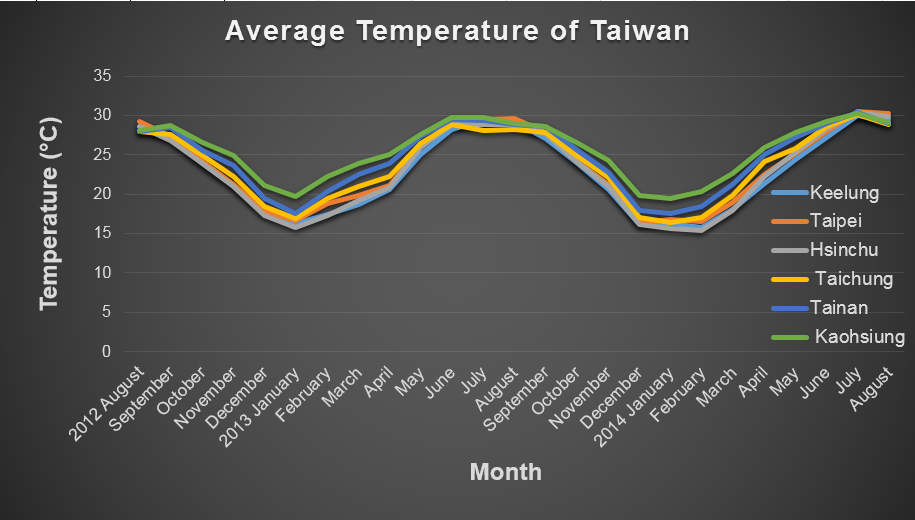
Temperature is key factor that can significantly influence the performance of our device, and it is hard to change the surrounding temperature if you place the device in the field. We need to take temperature into consideration. We, therefore, selected five temperatures between the highest and lowest average temperature last year (17.03 ℃ / 30.1 ℃) of Taipei for modeling.

Fig.3-2-1 Average temperature in Taiwan.
Experiment Data

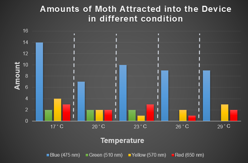
In the experiment part, we use CCW no.1 that we introduce in "Result/Insect Aspects" to evaluate the attracting ability of our device by changing the light wavelength and surrounding temperature. The insect would gather around a bottle based on their favor light color under consist temperature. This experiment is then repeated by changing the temperature from 17 to 29 degree Celsius. And the following table is our result.

Fig.3-3-1 The amount of moth attracted into oue device. Based on the result table, we can roughly find that blue light and 17 degree Celsius has the highest ability to attract insect. And the overall attraction ability is shown in our modeling result in Fig.3-3-3.
Fig.3-3-2 The result of our model in bar chart.

After experiment, the modeling using these data can simulate the capture ability in all conditions.

Fig.3-3-3 Simulating surface. The surface is composed of two conditional factor: surrounding temperature and light wavelength. And the surface can show the attraction ability in every temperature and light wavelength. This surface also means that user can know the attraction ability in any given condition which can significantly enhance the convenience of device usage.

The model of device aims to let the user easily input the condition value and know the device performance by this simulating surface. And the user can also find the local optima between the light wavelength 475 nm to 650 nm and the temperature between 17 to 29 degree Celsius.

Reference
  1. Central Weather Bureau of Taiwan http://stat.motc.gov.tw/mocdb/stmain.jsp?sys=100&funid=b8101

Modeling Software

MATLAB

MATLAB (matrix laboratory) is a numerical computing environment and fourth-generation programming language. It is developed by MathWorks, a company in United States. MATLAB allows matrix manipulations, plotting of functions and data, implementation of algorithms, creation of user interfaces, and interfacing with programs written in other languages, including C, C++, Java, and Fortran. Although MATLAB is intended primarily for numerical computing, an optional toolbox uses the MuPAD symbolic engine, allowing access to symbolic computing capabilities. An additional package, Simulink, adds graphical multi-domain simulation and Model-Based Design for dynamic and embedded systems.


Fig.4-1-1 MATLAB icon.
ANFIS

Adaptive-Network-Based Fuzzy Inference System, in short ANFIS, is a power tool for constructing a set of fuzzy if-then rules to generate stipulated output and input pairs. Unlike system modeling using mathematical rules that lacks the ability to deal with ill-defined and uncertain system, ANFIS can transform human knowledge into rule base, and therefore, ANFIS can effectively tune membership functions, minimizing the output error.