Team:Aachen/Notebook/Software/Measurarty

From 2014.igem.org

(Difference between revisions)
(Automatic Classification)
 
(4 intermediate revisions not shown)
Line 89: Line 89:
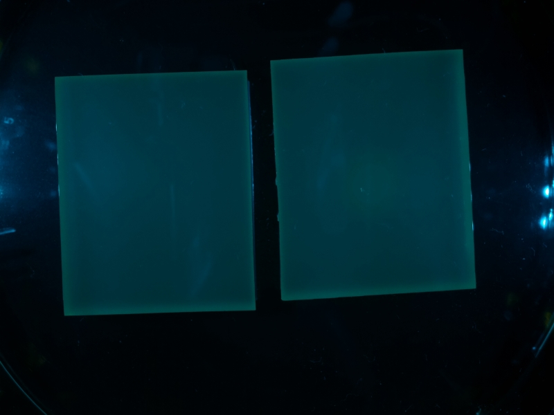
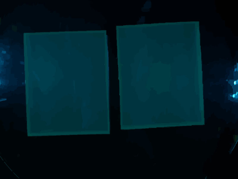
{{Team:Aachen/Figure|align=center|Aachen_meas_test.jpg|title=Image taken from WatsOn to be analyzed by ''Measurarty'' algorithm|width=700px}}
 +
{{Team:Aachen/BlockSeparator}}
Line 200: Line 201:
{{Team:Aachen/Figure|align=center|Aachen_meas_masked.png|title=Masked image|width=700px}}
 +
 +
{{Team:Aachen/BlockSeparator}}
Line 231: Line 234:
=== Empirical Evaluation ===
-
Using our MATLAB code we found the lower threshold for the smoothness index to be $TS_l = 0.85$ and the upper threshold $TS_u = \infty$.
+
Using our MATLAB code, we found the lower threshold for the smoothness index to be $TS_l = 0.85$ and the upper threshold $TS_u = \infty$.
Similarly, for $TI_l = 235$ and $TI_u = \infty$.
Using these settings, we can find a response already in images taken after 42 minutes.
-
Ideally, one would rate the quality of the image segmentation using some ground truth, such as manual delineations. This still has to be done for our method.
+
Ideally, one would rate the quality of the image segmentation using some ground truth, such as manual delineations. This still has to be implemented for our method.
However, from visual observations, our method is showing promising results.
Line 303: Line 306:
Combined with the input image, the final segmentation is received:
-
{{Team:Aachen/Figure|align=center|Aachen_meas_final.png|title=Final analyzed image|width=700px}}
+
{{Team:Aachen/Figure|align=center|Aachen_meas_final.png|title=Final the analyzed image|width=700px}}
[[File:Aachen_14-10-15_Medal_Cellocks_iNB.png|right|150px]]
[[File:Aachen_14-10-15_Medal_Cellocks_iNB.png|right|150px]]
 +
 +
{{Team:Aachen/BlockSeparator}}
Line 315: Line 320:
For example, changing from green to red fluorescence, only means to change the ''createMask'' function to select another target area.
-
Overall the results look convincing. We have not yet performed a comparison to a manual delineation, however, by eye the results look promising and have a low error.
+
Overall the results are convincing. We have not yet performed a comparison to a manual delineation, however, by eye the results look promising and have a low error.
Talking about computational complexity, the MATLAB code of course performs better than our own C++ implementation, which must be regarded as a proof-of-principle.
Line 357: Line 362:
* [https://static.igem.org/mediawiki/2014/6/6e/Aachen_measurarty.zip MATLAB code]
-
* link [https://github.com/orgs/igemsoftware/teams/aachen2014 github]
+
* link [https://github.com/igemsoftware/AachenSoftProject2014/tree/master/measurarty github]
For the C++ conversion please see [https://2014.igem.org/Team:Aachen/Notebook/Engineering/WatsOn#watsonsoftware our ''WatsOn'' Software] section.

Latest revision as of 03:46, 18 October 2014

Measurarty

Measurarty is the evil player in the game of Cellock Holmes and WatsOn. Measurarty is the pathogen detection logic behind our project. Using our Measurarty algorithm, we want to automatically detect pathogens from the chip photos delivered by WatsOn, without human interaction. Besides reducing the risk of human errors, this makes our device usable by almost everyone.


Aachen Measurarty Intro button.png

Measurarty - An Introduction

Our device control software is able to take images of incubated chips inside WatsOn. Yet, that does not bring the user closer to the answer of the question:

What's on the chip?

In fact, answering this question seems trivial for a human: Just check whether a colony grown has grown on the chip and you're done. This task is even easier with our chip system, because these show fluorescence wherever a pathogen has been detected.

But is this an easy task for a computer? Actually not. The task of automatic detection is tried by several disciplines in computer science, from pattern recognition over machine learning to by medical imaging chairs.

Here, we would like to present a pipeline for this task that makes use of easy segmentation and classification algorithms. First, Measurarty segments the target image using Statistical Region Merging (SRM) in order to find regions of similar properties. After this step, we can segment the picture using histogram thresholding in [http://en.wikipedia.org/wiki/HSL_and_HSV HSV color space] to find candidate regions for pathogens. Finally, a classification algorithm can detect the pathogen on our chips.

To demonstrate the algorithm, the following sample image will be discussed.

Aachen meas test.jpg
Image taken from WatsOn to be analyzed by Measurarty algorithm


Aachen Puzzels button.png

Statistical Region Merging (SRM)

Before briefly introducing Statistical Region Merging (SRM), we would like to explain why we need this step, and why this algorithm is an ideal choice.

Compared to other clustering algorithms, SRM is quite leight weight, yet delivers deterministic results and is not dependent on a certain seed (like k-means, for example).

On the other hand, it can create as many refinements as one wants and is thus flexible enough for the our purposes. Finally, there's already been knowledge about this algorithm in the group.

Statistical Region Merging (SRM) (Nook and Nielson, 2004) is a clustering technique also used directly for image segmentation. A region $R$ is a set of pixels and the cardinality $\lvert R \rvert$ determines how many pixels are in one region. Starting with a sorted set of connected regions (w. r. t. some distance function $f$), two regions $R$ and $R'$ are merged if the qualification criteria $\vert \overline{R'}-\overline{R} \vert \leq \sqrt{b^2(R)+b^2(R')}$ with $b(R) = g \cdot \sqrt{\frac{\ln \frac{\mathcal{R}_{\lvert R \rvert}}{\delta}}{2Q\lvert R \rvert}}$ is fulfilled. Therefore, $\mathcal{R}_{\lvert R \rvert}$ is the set of regions with $\lvert R \rvert$ pixels. Typically $Q$ is chosen as $Q \in \lbrack 256, 1\rbrack$ and $\delta = \frac{1}{\lvert I \rvert^2}$.

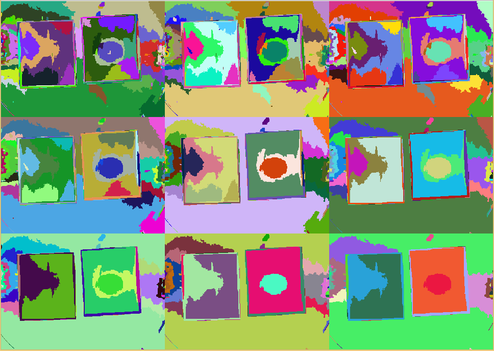
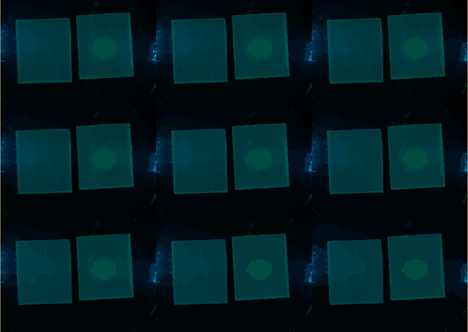
The $Q$ parameter mainly influences the merging process. For an example, see the figure SRM Regions below. The lower the chosen value for $Q$, more coarse the regions become. Using a union-find structure, the segmentation does not need to be recalculated for each $Q$ level. For the step from $q$ to $\frac{q}{2}$, just the qualification criteria needs to be applied to the regions from the $q$ result. A MATLAB implementation is also available (Boltz, 2009).

Aachen srm regions 3.PNG Aachen srm regions 2.PNG
SRM regions in random colors
Different regions from an SRM run starting at $Q=256$ (top left) and going to $Q=1$ (bottom right). Each region is assigned a random color.
SRM regions (average color)
Different regions from an SRM run starting at $Q=256$ (top left) and going to $Q=1$ (bottom right). Each region is assigned the average color of that region.

SRM Clustering

In our project, we used Statistical Region Merging for clustering. In contrast to other algorithms, such as k-means, this approach is highly deterministic. For our purposes we only have one SRM run for $Q=256$.

In MATLAB, we use the previously mentioned code from MATLAB Fileexchange (Boltz, 2009). For our Qt-based GUI we implemented the SRM method ourselves.

The SRM clustering reduces the amount of different colors in the image and hence eases the recognition of parts belonging together.


Qlevel = 256;
[maps,images]=singlesrm(double(image),Qlevel);

Finally, if applied to our test-image, regions are created and homogenoues regions form:

Aachen meas srmed.png
Regions created with SRM clustering


Aachen SEgment button.png

Segmentation

In the segmentation stage all background regions are removed. This task is quite crucial. If one removes too few, the final stage of finding pathogens might get irritated. On the other hand, if one removes too many regions, positive hits might get removed early before detection. This surely must be avoided.

We opted for a simple thresholding step because it showed that while being easy, it is an effective weapon against the uniform background. In fact, the good image quality we wanted to reach with our device allows now less sophisticated methods. Also the less computational intensive the steps are, the better they might even run directly on the Raspberry Pi in our device!

The HSV thresholding is performed on each component seperately. For more information on the HSV color space we refer to [http://en.wikipedia.org/wiki/HSL_and_HSV Wikipedia]. The first component is the hue which we select to be inbetween $0.462$ and $0.520$ to select any blue-greenish color. We will not see bright green due to the filter selection in our device. The saturation value must be high, between $0.99$ and $1.0$. Moreover, the value component of the HSV image has to lie between $0.25$ and $0.32$, which assumes a relatively dark color.

Indeed, these values are not problem specific, but specific for each setup and therefore have to be determined empirically.

The remainder of this stage creates a mask of pixels that fulfill the conditions.


% Auto-generated by colorThresholder app on 15-Oct-2014
%-------------------------------------------------------
function [maskedRGBImage] = createMask(srmimg)
RGB = srmimg;

% Convert RGB image to chosen color space
I = rgb2hsv(RGB);

% Define thresholds for channel 1 based on histogram settings
channel1Min = 0.462;
channel1Max = 0.520;

% Define thresholds for channel 2 based on histogram settings
channel2Min = 0.99;
channel2Max = 1.000;

% Define thresholds for channel 3 based on histogram settings
channel3Min = 0.25;
channel3Max = 0.32;

% Create mask based on chosen histogram thresholds
BW = (I(:,:,1) >= channel1Min ) & (I(:,:,1) <= channel1Max) & ...
    (I(:,:,2) >= channel2Min ) & (I(:,:,2) <= channel2Max) & ...
    (I(:,:,3) >= channel3Min ) & (I(:,:,3) <= channel3Max);

% Initialize output masked image based on input image.
maskedRGBImage = RGB;

% Set background pixels where BW is false to zero.
maskedRGBImage(repmat(~BW,[1 1 3])) = 0;

end

If you apply this HSV masking code to the SRMed test image, the following is created:

Aachen meas masked.png
Masked image


Aachen Classify button.png

Classification

Smoothness Index

For position prediction in virtual environments, jitter or noise in the output signal is not wanted though often present. Since discovering smooth areas is a similar problem to jitter detection, a simple method for determining jitter can be used to measure non-jitter, smoothness (Joppich, Rausch and Kuhlen, 2013). It is assumed that jitter-free areas of a position signal do not differ in velocity.

Smooth areas do not differ in intensity, and therefore only low changes in velocity (intensity change) can be recorded. For the reduction of noise, this operation is performed on the smoothed input image. Then the smoothness $s$ of a pixel $p$ in its k-neighbourhood $\mathcal{N}_k$ can be determined as: \begin{equation} s(p) = \sum\limits_{p' \in \mathcal{N}_k} \nabla(p') / \arg\max\limits_{p} s(p) \end{equation}

Using thresholding, $TS_l \leq s(p) \leq TS_u \wedge TI_l \leq I \leq TI_u$, different areas, such as background or pathogen, can be selected.

For the empirical choice of thresholds, it can be argued that these are tailored to the specific case. While this surely is true to a certain extent, the here presented method has been successfully tested on images from a completely different domain, and no changes to the thresholds have been made to make it work. A proper theoretical evaluation is emphasized, however, is probably not the aim of the iGEM competition.

Finally, selecting for the red region, this delivers the location of possible pathogens. Since the size of the agar chips is variable but fixed a quantitative analysis can be performed by counting pixels for instance.

Empirical Evaluation

Using our MATLAB code, we found the lower threshold for the smoothness index to be $TS_l = 0.85$ and the upper threshold $TS_u = \infty$. Similarly, for $TI_l = 235$ and $TI_u = \infty$.

Using these settings, we can find a response already in images taken after 42 minutes.

Ideally, one would rate the quality of the image segmentation using some ground truth, such as manual delineations. This still has to be implemented for our method. However, from visual observations, our method is showing promising results.

  • image of smoothness index

Automatic Classification


function [mask, seg] = automaticseeds(im)

    imc = im;

    %% to grayscale and filtering
    Z = double(rgb2gray(im));
    Z = 255 * Z / max(max(Z));

    filtertype = 'disk';
    Z = filter2(fspecial(filtertype), Z);
    Z = filter2(fspecial(filtertype), filter2(fspecial(filtertype), Z));
    Z = 255 * Z / max(max(Z));   
    
    %% calculating similarity score/smoothness index
    k=4;
    sSI = similarity(Z,k);
    sSI = sSI / max(max(sSI));  
    
    %% classify
    pathogene = ((sSI > 0.85) == 1) & ((Z > 235) == 1);  

    mask = ones( size(imc) );
    seg = zeros( size(imc) );

    
    %% output
    for i=1:size(im,1)
        for j=1:size(im,2)
            
            if (pathogene(i,j) == 1)
                seg(i,j,1:3) = [255 0 0];
                mask(i, j, 1:3) = [0 0 0];
            end
        end
    end
end

This code actually creates two intermediate images from which the similarity index is calculated. First the smoothed (disk-filter) input image is created and stored:

Aachen meas smoothed.png
Smoothed image

Only white regions are candidate regions. After smoothing, the similarity index is calculated. As expected, edges are detected and limit the area from which the target region can be selected.

Aachen meas smiliarity.png
Smoothness Index

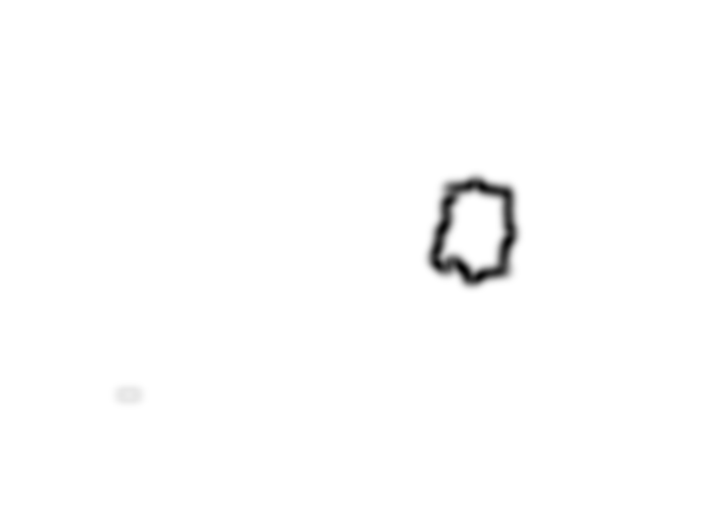
Finally the selected pathogen region is selected by the black area in the following picture:

Aachen meas mask.png
Selected region

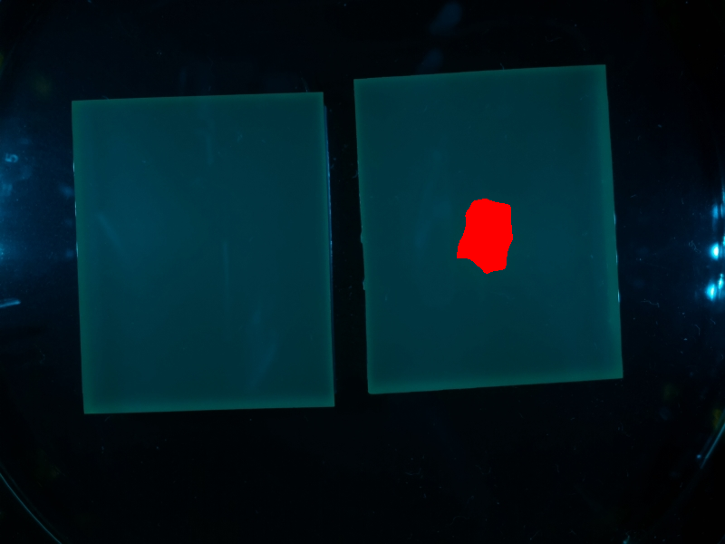
Combined with the input image, the final segmentation is received:

Aachen meas final.png
Final the analyzed image
Aachen 14-10-15 Medal Cellocks iNB.png


Achievements

Measurarty is the image analysis logic behind our project. It is comprised of simple constructs put together into a pipeline, that is clearly laid out, easily maintainable and - if needed - easily adaptable. For example, changing from green to red fluorescence, only means to change the createMask function to select another target area.

Overall the results are convincing. We have not yet performed a comparison to a manual delineation, however, by eye the results look promising and have a low error.

Talking about computational complexity, the MATLAB code of course performs better than our own C++ implementation, which must be regarded as a proof-of-principle.

Space-wise, the code depends heavily on the image size $O( x \cdot y)$ (width $x$, height $y$, which also limits the number of edges in SRM between regions, as each pixel is one region to start with. However, it cannot take less memory, as the image is stored in an uncompressed format.

On the computational side, the thresholding, image conversion and gradient steps are linear in the number of pixels, and are thus in $O(x \cdot y)$. Unfortunately, the summation of the gradient for the smoothness index adds a heavy factor to it (k-neighbourhood for smoothness index). Due to the merging step in our C++-SRM algorithm implementation, our code has to do $O(x^2 \cdot y^2)$ comparisons, which then finally results in a runtime complexity of $O( x^2 \cdot y^2)$.

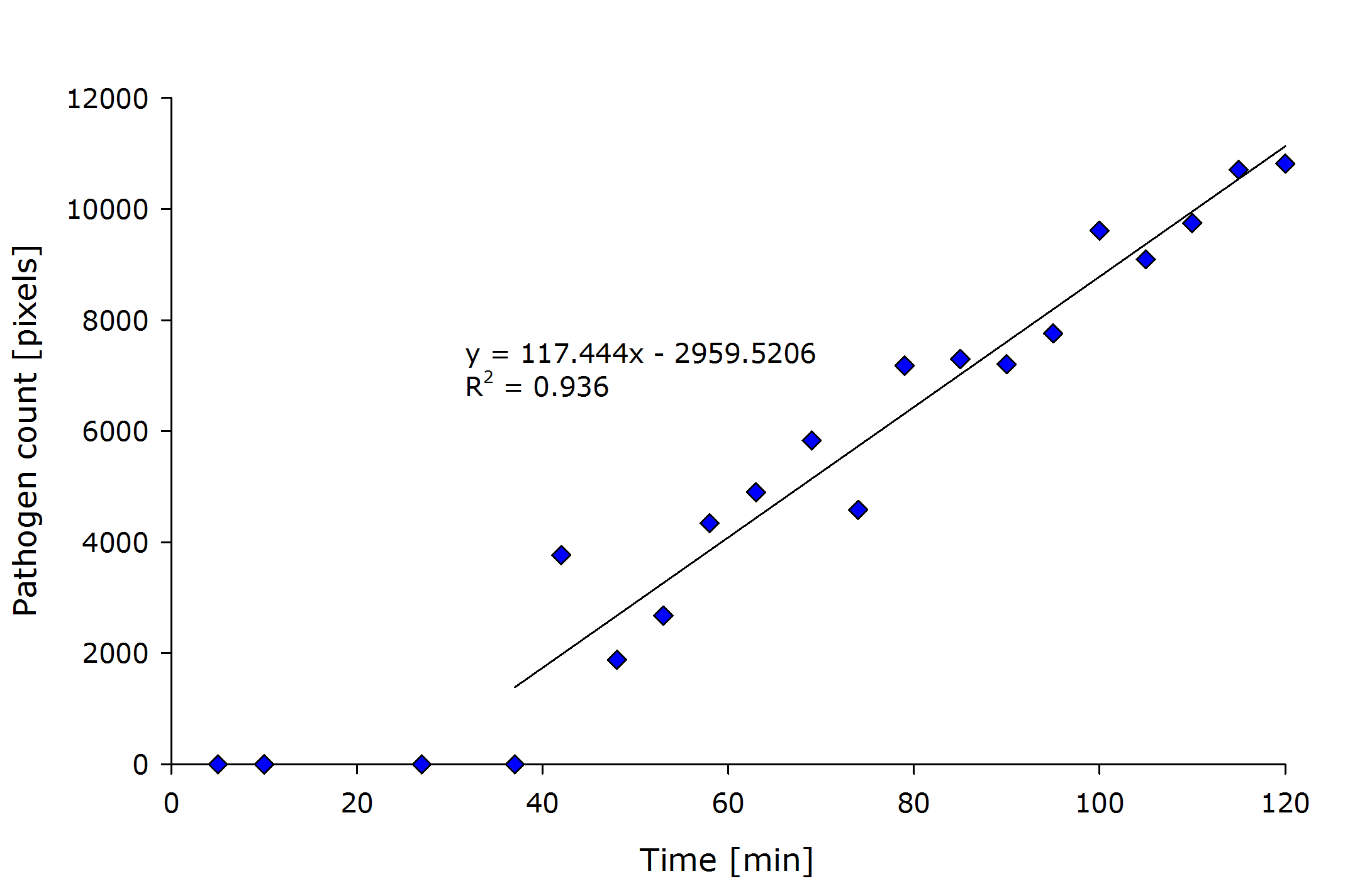
Aachen meas sizes.png
Pixel count of the detected pathogenic region versus time after induction.

From the above figure it can also be seen that the detected amount of pathogenic-area correlates with time after induction. The lag-phase can be explained first by the lag-phase of the cells, which first need to generate a response to the pathogen, and on the other hand, by too low fluorescence which is not detectable. The pixel count also meets the expectation when looking at the sample files by eye.

Detecting P. aeroginosa with K131026
The left half shows the original images from the device and the right half shows the same pictures with the detected pathogenic region analyzed by Measurarty.

It can be concluded that the Measurarty pipeline defines a robustly working chip-analysis algorithm which can detect pathogens from images supplied by WatsOn. Therefore, this algorithm closes the gap between our biology, detection hardware and the user who wants easy-to-interpret results.

For future prospects, it would be interesting to do a proper performance analysis on our code, to find hotspots and optimize the code. Many for-loops leave plenty of room for vectorization and loop-unrolling. Parallelization, specifically with respect to embedded hardware such as the Raspberry Pi or Odroid U3, is limited to the extend that the overhead created would probably eliminate the improvements.


Source Code

Measuarty is the image analysis logic behind our project. It has been prototyped and developed in [http://www.mathworks.de/academia/student-competitions/igem/ MATLAB], and only later been ported into our WatsOn GUI.

We are happy to provide you with a zip-ped download of our MATLAB code here, as well as on the iGEM software repository on github.

For the C++ conversion please see our WatsOn Software section.

Using the MATLAB Code

In general, please follow the included README.MD file. Our package comes with a set of test files from one of our experiments. After installing the Statistical Region Merging code (see readme), you can simply run igem_srm_demo.m. Select your current folder, and MATLAB will automatically segment and classify the included jpg-images.


References

  • Boltz, S. (2009, October 20). Image segmentation using statistical region merging - File Exchange - MATLAB Central. Image segmentation using statistical region merging. Retrieved December 12, 2013, from http://www.mathworks.com/matlabcentral/fileexchange/25619-image-segmentation-using-statistical-region-merging
  • Joppich, M., Rausch, D., & Kuhlen, T. (2013). Adaptive human motion prediction using multiple model approaches.. Virtuelle und erweiterte Realität (p. 169–180). 10. Workshop der GI-Fachgruppe VR/AR: Shaker.
  • Nock, R., & Nielsen, F. (2004). Statistical region merging. IEEE Transactions on Pattern Analysis and Machine Intelligence, 26(11), 1452-1458.