Team:ETH Zurich/labblog/20140824mod
From 2014.igem.org
(Created page with "<html><article class="mix carousel modeling parameter qsmodule" id="qsdynamics" date="20140824"></html> == Fitting quorum sensing dynamic curves == ==== Monday, August 24th ===...") |
(→Monday, August 24th) |
||
| (6 intermediate revisions not shown) | |||
| Line 7: | Line 7: | ||
$$\frac{d[GFP]}{dt}=\frac{k_{45}[P_{tot}]\Big(-1+\sqrt{1+8\frac{AHL_i}{K_{d3}}}\Big)^2}{16\frac{K_{d4}}{K_{d3}}+\Big(-1+\sqrt{1+8\frac{AHL_i}{K_{d3}}}\Big)^2}-d_{GFP}[GFP]$$. | $$\frac{d[GFP]}{dt}=\frac{k_{45}[P_{tot}]\Big(-1+\sqrt{1+8\frac{AHL_i}{K_{d3}}}\Big)^2}{16\frac{K_{d4}}{K_{d3}}+\Big(-1+\sqrt{1+8\frac{AHL_i}{K_{d3}}}\Big)^2}-d_{GFP}[GFP]$$. | ||
For very high initial concentrations AHLi, we have | For very high initial concentrations AHLi, we have | ||
| - | + | $$\frac{d[GFP]}{dt}=k_{45}[P_{tot}]-d_{GFP}[GFP]$$ | |
| - | so by taking $t_{1/2}=\frac{ln(2)}{d_{GFP}}$ from experimental curves, we are able to retrieve $$d_{GFP} = 4.9 . 10^{-3} min^{-1}$$. | + | so by taking |
| + | |||
| + | $$t_{1/2}=\frac{ln(2)}{d_{GFP}}$$ | ||
| + | |||
| + | from experimental curves, we are able to retrieve | ||
| + | |||
| + | $$d_{GFP} = 4.9 . 10^{-3} min^{-1}$$. | ||
For very low initial concentrations of initial AHL and considering degradation, we have | For very low initial concentrations of initial AHL and considering degradation, we have | ||
| - | $$\frac{d[GFP]}{dt}=\frac{k_{45}[P_{tot}][AHLi]^2e^{-2d_{AHL}t}}{K_{d4}K_{d3}}-d_{GFP}[GFP]$$ | + | $$ \frac{d[GFP]}{dt}=\frac{k_{45}[P_{tot}][AHLi]^2e^{-2d_{AHL}t}}{K_{d4}K_{d3}}-d_{GFP}[GFP].$$ |
| - | We find $$[GFP]=\frac{k_{45}[P_{tot}][AHLi]^2}{K_{d4}K_{d3}(d_{GFP}-2d_{AHL})}(e^{-2d_{AHL}t}-e^{-d_{GFP}t})$$ | + | We find |
| + | $$ [GFP]=\frac{k_{45}[P_{tot}][AHLi]^2}{K_{d4}K_{d3}(d_{GFP}-2d_{AHL})}(e^{-2d_{AHL}t}-e^{-d_{GFP}t}).$$ | ||
This curve has a maximum at | This curve has a maximum at | ||
| - | $$t_{max}=\frac{1}{d_{GFP}-2d_{AHL}}ln\big(\frac{d_{GFP}}{2d_{AHL}}\big)$$ | + | $$ t_{max}=\frac{1}{d_{GFP}-2d_{AHL}}ln\big(\frac{d_{GFP}}{2d_{AHL}}\big).$$ |
| - | + | This way we can find from experimental curves $$d_{AHL}=4,0.10^{-3} min^{-1}$$ | |
| + | |||
| + | This AHL degradation rate is alumped parameter between internal and external degradation rates, equivalent to | ||
| + | |||
| + | $$d_{AHLext}+\alpha d_{AHLint}$$ | ||
| - | + | where α is the fraction of the volume occupied by cells in the whole culture. From that on we could find reasonable values for internal and external AHL degradation rates. | |
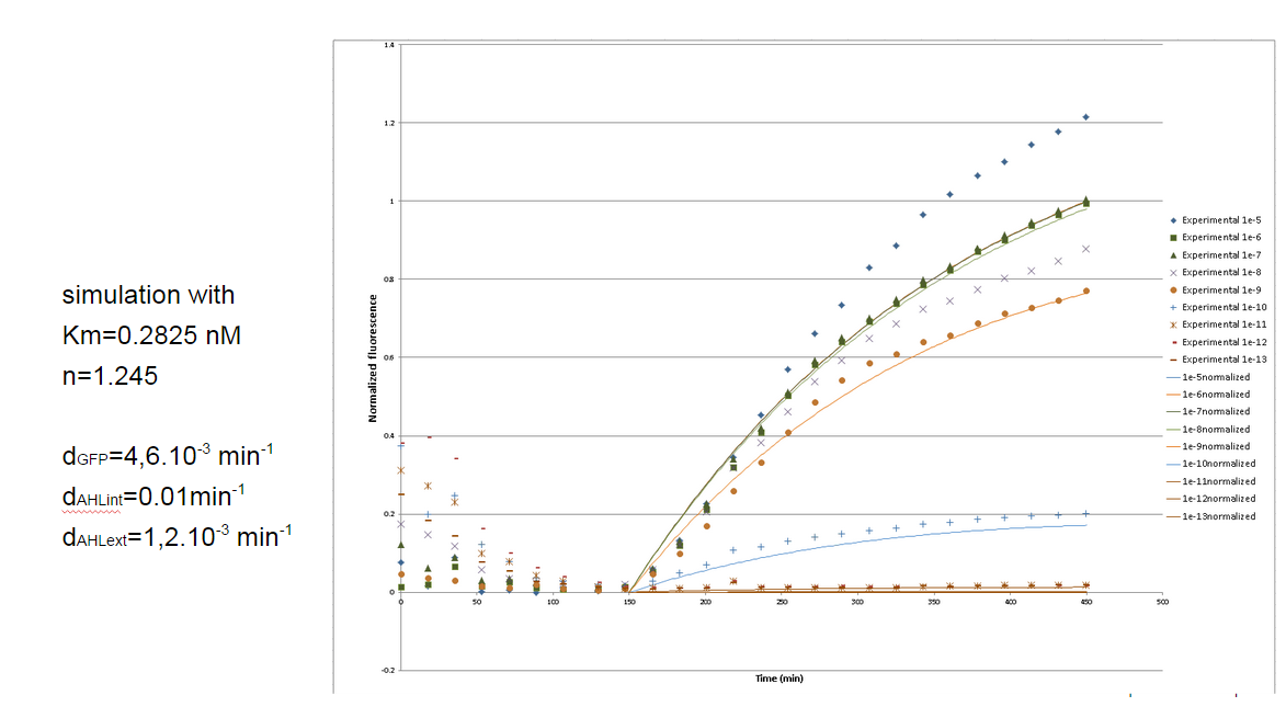
Finally the curves simulated by our model with these parameters fit the experiments quite well: | Finally the curves simulated by our model with these parameters fit the experiments quite well: | ||
Latest revision as of 20:04, 11 October 2014
Fitting quorum sensing dynamic curves
Monday, August 24th
We could use quorum sensing dynamic curves to fit degradation rates of external, internal AHL and GFP. We fitted the experimental results for lux with riboregulator and thus didn't consider leakiness (we showed leakiness was low enough in that case when fitting quorum sensing Hill function parameters ). By writing GFP production rate and replacing AHL in this equation by $$[AHL]=[AHL_i]-[AHL_{bound}]$$ we find $$\frac{d[GFP]}{dt}=\frac{k_{45}[P_{tot}]\Big(-1+\sqrt{1+8\frac{AHL_i}{K_{d3}}}\Big)^2}{16\frac{K_{d4}}{K_{d3}}+\Big(-1+\sqrt{1+8\frac{AHL_i}{K_{d3}}}\Big)^2}-d_{GFP}[GFP]$$. For very high initial concentrations AHLi, we have $$\frac{d[GFP]}{dt}=k_{45}[P_{tot}]-d_{GFP}[GFP]$$
so by taking
$$t_{1/2}=\frac{ln(2)}{d_{GFP}}$$
from experimental curves, we are able to retrieve
$$d_{GFP} = 4.9 . 10^{-3} min^{-1}$$. For very low initial concentrations of initial AHL and considering degradation, we have
$$ \frac{d[GFP]}{dt}=\frac{k_{45}[P_{tot}][AHLi]^2e^{-2d_{AHL}t}}{K_{d4}K_{d3}}-d_{GFP}[GFP].$$
We find
$$ [GFP]=\frac{k_{45}[P_{tot}][AHLi]^2}{K_{d4}K_{d3}(d_{GFP}-2d_{AHL})}(e^{-2d_{AHL}t}-e^{-d_{GFP}t}).$$
This curve has a maximum at
$$ t_{max}=\frac{1}{d_{GFP}-2d_{AHL}}ln\big(\frac{d_{GFP}}{2d_{AHL}}\big).$$
This way we can find from experimental curves $$d_{AHL}=4,0.10^{-3} min^{-1}$$
This AHL degradation rate is alumped parameter between internal and external degradation rates, equivalent to
$$d_{AHLext}+\alpha d_{AHLint}$$
where α is the fraction of the volume occupied by cells in the whole culture. From that on we could find reasonable values for internal and external AHL degradation rates.
Finally the curves simulated by our model with these parameters fit the experiments quite well:
 "
"
