 "
"
Team:Valencia UPV/Modeling/gene expresion
From 2014.igem.org
| Line 1: | Line 1: | ||
{{:Team:Valencia_UPV/header}} | {{:Team:Valencia_UPV/header}} | ||
| - | <1-- | + | <html><1-- |
<ul class="nav nav-tabs" id="myTab"> | <ul class="nav nav-tabs" id="myTab"> | ||
<li class="active"><a href="#Devices_Overview">Devices Overview</a></li> | <li class="active"><a href="#Devices_Overview">Devices Overview</a></li> | ||
| Line 432: | Line 432: | ||
}); | }); | ||
</script> | </script> | ||
| - | </html | + | --></html> |
{{:Team:Valencia_UPV/footer_img}} | {{:Team:Valencia_UPV/footer_img}} | ||
Revision as of 19:03, 6 September 2014
Group behavior
One of the 3D simulations performed in SciLab.
In practice, a single C. elegans is not employed to perform the task but a group of worms. In this case, the random walk equations obtained for a single worm behavior can be transformed into partial differential equations (PDEs), using Taylor series, to depict the distribution of the population, as the ones describing a diffusion process (![]() Click here for a mathematical proof of one dimensional diffusion process using PDEs from random walk)
Click here for a mathematical proof of one dimensional diffusion process using PDEs from random walk)
However, in our case we face a diffusion system with drift, in which the last term arises from the biased movement of C. elegans. To obtain a PDE that reflects this behavior, we employed difference equations also using Taylor series and apropiate limits (![]() Click here for a mathematical proof of two dimensional biased diffusion process (C. elegans chemotaxis behavior) using PDEs from biased random walk)
Click here for a mathematical proof of two dimensional biased diffusion process (C. elegans chemotaxis behavior) using PDEs from biased random walk)
The equation is the following:
$$\frac{\partial [C]}{\partial t} = D\;\nabla^2[C] - \nabla\cdot(\underline{\nu}\;[C]) $$
Once obtanied the equation that governs our system, we proceed to study if it works correctly for our purpose. However, analytical solutions for this equation are known for few ideal cases. For example, for a monodimensional bistable potential the stationary state is the following (Okopinska, 2002):
$$ P_{ss}=\mathscr{N}^{-1} e^{\left(-V(x)/D\right)}$$ where $ \mathscr{N} $ is the normalization constant.

As seen, our system, can theoretically work as expected, depending on the shape of the chemoattractant only. This is a great result because it shows our worms are capable of reaching each region.
Our final goal in this section is predicting the temporal and spatial behavior in 2D for non-ideal problems. In this case, using numerical methods is the only way to solve the system.
For the 2-dimensional case, $[C] = [C(x, y, t)]$ is the concentration of C. elegans at a given instant $t$ and at a given point $(x, y)$, $D$ is the diffusion coefficient and $\overrightarrow{\nu}$ is the attraction field for the C. elegans, which basically stands for its velocity. This expression naturally expands to: $$\frac{\partial [C]}{\partial t} = D \; \left(\frac{\partial^2 [C]}{\partial x^2} + \frac{\partial^2 [C]}{\partial y^2}\right) - \left(\frac{\partial\nu_x}{dx}[C] + \nu_x\frac{\partial [C]}{\partial x} + \frac{\partial\nu_y}{dy}[C] + \nu_y\frac{\partial [C]}{\partial y}\right) $$
We first started by building up an explicit finite difference method, this is numerically fast but it is prone to instabilities in the solutions. Therefore, we decided to develop a Crank-Nicolson method which is unconditionally stable, thus being suitable to carry out parameter identification of a model. Nevertheless, it has the drawback of being numerically more intensive, because a set of algebraic equations must be solved in each iteration (![]() Click here for a mathematical explanation of the Crank-Nicolson method).
Click here for a mathematical explanation of the Crank-Nicolson method).
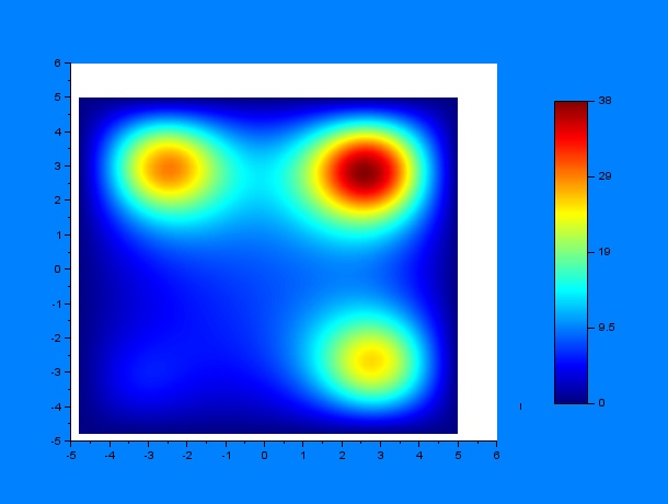
Now, we can predict the behavior of a set of worms in presence of a chemoatractant. One must have into account that the system may behave differently depending on some variables, for example, the diffusion coefficient $D$, a constant $k$ that determines the weight that the drift variable $\nu$ has and the time constants for the chemoattractant diffusion $t_1$ and $t_2$, where $t_1$ is the elapsed time since a first chemoattractant drop is put into the petri plate, $t_2$ stands for the elapsed time since a second drop of chemoattractant is put into the petri plate until a C.elegans initial distribution is added, the diffusion of chemoattractants is then assumed to be negligible for simplicity reasons. According to these parameters, we performed a lot of simulations using SciLab, what they all have in common is the position of the four chemotactic sources. The simulations were performed by first varying only $t_1$ and $t_2$ for some given $D$ and $k$ ($D = 0.2$ & $k = 0.001$):
 $t_1$ = 5, $t_2$ = 6
 $t_1$ = 5, $t_2$ = 12
 $t_1$ = 10, $t_2$ = 12
 $t_1$ = 10, $t_2$ = 24
 $t_1$ = 15, $t_2$ = 24
 $t_1$ = 15, $t_2$ = 48
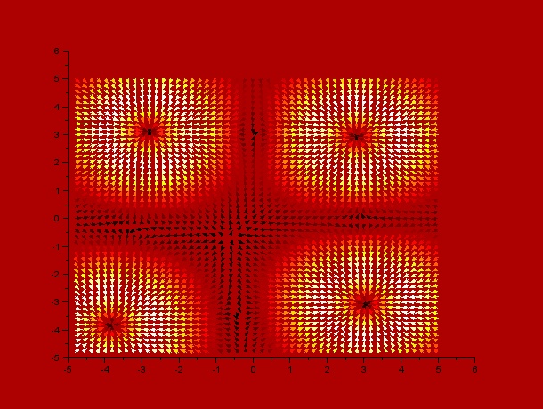
It can be observed by ploting the drift field for each case, that the final distribution is mostly dependent on the mentioned drift field, which in fact is mostly dependent on $t_1$ and $t_2$. Here we present the drift fields for each case:
 $t_1$ = 5, $t_2$ = 6
 $t_1$ = 5, $t_2$ = 12
 $t_1$ = 10, $t_2$ = 12
 $t_1$ = 10, $t_2$ = 24
 $t_1$ = 15, $t_2$ = 24
 $t_1$ = 15, $t_2$ = 48
Qualitatively, it can be seen through these simulations that incrementing $t_1$ or $t_2$ disperses and smoothes the drift field which actually affects the final distribution of C.elegans by dispersing it.
Videos corresponding to each simulation can also be seen here:
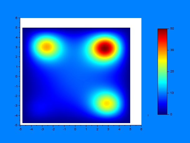
And then by varying only $D$ and $k$ (separately, of course) for some given $t_1$ and $t_2$ ($t_1 = 10$ hours & $t_2 = 12$ hours):
 D = 0.05, k = 0.001, D/k = 50
 D = 0.1, k = 0.001, D/k = 100
 D = 0.2, k = 0.001, D/k = 200
 D = 0.05, k = 0.0005, D/k = 100
 D = 0.1, k = 0.0005, D/k = 200
 D = 0.2, k = 0.0005, D/k = 400
According to these results, qualitatively, higher values of $D$ or lower values of $k$ (and thus a greater $D/k$ relation) give a much more disperse distribution of C.elegans.
Videos corresponding to each simulation can be seen here:
We also carried out some simulations with different number of attractant sources. One can find simulations with $1$, $2$ and $3$ sources, and parameters $D\;=\;0.2$, $k\;=\;0.001$ (thus $D/k\;=\;200$) here:
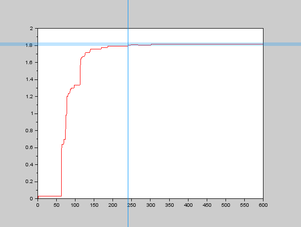
Parameter identification in PDEs is a rather complex topic, we did some research concerning our Group Behavior Model which is a Fokker-Planck Equation with a somewhat complex drift term $\nu$, which depends on position in our model (it could also depend on more factors which would add even more complexity to the system and therefore we didn't study them). We weren't lucky enough to find anything related to the topic (at least with the time we had), so we thought about implementing our own algorithms, based on an educated guess (As usual all the code we wrote can be found under the Software section). We wanted to study the spatial time constant of the system, that is, how long does it take for the system to reach an stable spatial distribution? We thought about a obtaining a variable $\mathcal{V}$ that would grow asimptotically after some time $\tau_{xy}$ (the spatial time constant). That is, our variable $\mathcal{V} \rightarrow C$ as $\tau_{xy} \rightarrow +\infty$. We then came up with the idea that local maxima would be a good way to define when the spatial distribution was stable, so we decided that the slower local maximum (that is the local maximum which is the slowest in stabilizing to its final position) would be a good approach to define the spatial time constant $\tau_{xy}$.
Therefore we needed an algorithm to calculate all the local maxima at a given instant and also to determine when they have "stopped" moving, so we programmed an approximate algorithm to find the local maxima in SciLab and used a more or less small band centered around the final value to determine $\tau_{xy}$. An example of the graphs we obtained through this process can be seen here:
So we carried out several simulations with different values for our parameters $D$ and $k$, in order to obtain the forementioned relationship between $D$, $k$ and $\tau_{xy}$.
First of all, we managed to plot and obtain the function that relates $D$ with $\tau_{xy}$, for $k=0.00025,\;0.0003,\;0.000375,\;0.0005$ and $0.001$. And as one can observe, different values of $k$ just move the curves but the main shape of the functionals remains the same, that is, exponential (with rather great coefficients of determination).

From the results we hypothesized that the general form of the functional (depending on $k$) was as follows:
$$D(\tau_{xy},k) = f(k)e^{\left(g(k)\tau_{xy}\right)}$$
We then plotted the coefficients $f(k)$ and $g(k)$ vs. $k$, as shown here:

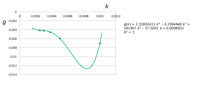
We first obtained a quadratic regression and the resulting equations for $f(k)$ and $g(k)$ were:
$$f(k) = 3e6\;k^2 - 4658.1\;k+1.9523$$
$$g(k) = 6177.4\;k^2 - 11.907\;k-0.0013$$
But $R^2$ was about $80.17\%$ for $f(k)$, way too low, so then we decided to obtain a better model by using Lagrange's Interpolating Polynomials, which are represented by the green curves on the graphs above. Thus we obtained the following final equation for $D$:
$$D(\tau_{xy},k) = \left(-3.4061e13\;k^4+4.22776e10\;k^3+3.2955e6\;k^2-15277\;k+4.19004 \right)\;e^{\left(2.31802e11\;k^4-4.23644e8\;k^3+241467\;k^2-57.5001\;k+0.0008832 \right)\;\tau_{xy}}$$
From this the equation for $\tau_{xy}$ can be obtained:
$$\tau_{xy}(D,k) = \frac{1}{0.0008832 - 57.5001\; k + 241467\; k^2 - 4.23644e8\; k^3+2.31802e11\; k^4} log\left(\frac{D}{4.19004 - 15277\; k + 3.2955e6\; k^2 + 4.22776e10\; k^3 - 3.4061e13\; k^4}\right)$$
Where $D$ and $k$ are the mentioned parameters of the model and $\log$ refers to the natural logarithm (base $e$).
The average of the relative error is somewhat lower (at least in the studied region), about $8.00677\%$, compared to about $9.4\%$ for the first approximation.
From this equations we tried to obtain the parameters $D$ and $k$ for our model by stablishing a relationship that would not lead to dirac deltas in the final solution, which is what usually happened and is the theoretical solution provided the initial distribution of worms is also a dirac delta. Therefore we obtained the relationship $\frac{D}{k} = 502.2$ that would lead to a temporal stabilisation of the distribution, meaning no dirac deltas would arise. The intention was to provide our wetlab mates with theoretical data to improve their experiments and therefore creating a feedback loop in which they could provide data to us to improve our model even more and they would receive result back and so on. But, in fact, with the obtained relationship and our data we weren't able to find correct values for $D$ and $k$. We think this maybe due to the restricted region for $\tau_{xy}$, $D$ and $k$ that we studied. We also think that through the same process we would be able to achieve correct relationships for the variables in other regions of interests the problem is with increasingly small $D$ and $k$ parameters, come increasingly large times for the simulations to run and we weren't able to do so in our personal computers. This would therefore be a future task, to carry out more simulations maybe on a computer cluster with parallelization. We think that then the principles we followed would still hold.
Okopinska A. (2002) Fokker-Planck equation for bistable potential in the optimized expansion. Physical review E, Volume 65, 062101
-->