 "
"
Team:Heidelberg/pages/Linker Modeling
From 2014.igem.org
(Created page with "=General= During the iGEM competetion we have written a software, that can predict the best linker to circularize a protein. Therefore at first connections between the ends are f...") |
(→In silico refinement) |
||
| (88 intermediate revisions not shown) | |||
| Line 1: | Line 1: | ||
| - | = | + | =Background= |
| - | + | Primary, secondary, tertiary and quaternary structures are the main levels of protein structure characterization. Primary structure designates the amino acid sequence, while the secondary structure describes the arrangement of consecutive amino acids through their two dihedral angles $\phi$ and $\psi$. The Ramachandran plot, which represents the amino acid position in the space of those two angles, shows two particular arrangement commonly found in proteins: alpha helices and beta sheets. The next level of protein organization is the tertiary structure, which describes how the protein is organized in the three spatial dimensions, whereas the quaternary structure describes how different subunits of proteins cluster. | |
| - | + | Finally, closely related to these standard structures, the supersecondary structure describes how secondary structure elements are connected to each other. While these connections look undefined at first sight, further analysis revealed that this wide variety of supersecondary structure motifs can be clustered to certain patterns [[#References|[5]]]. | |
| - | + | ||
| - | + | ||
| - | + | ||
| - | + | ||
| - | + | ||
| - | + | ||
| - | + | ||
| - | + | ||
| - | + | ||
| - | + | ||
| - | + | ||
| - | + | ||
| - | + | ||
| - | + | ||
| - | + | ||
| - | + | ||
| - | + | ||
| - | + | ||
| - | + | ||
| - | + | ||
| - | + | ||
| - | + | ||
| - | + | ||
| - | + | ||
| - | + | ||
| - | + | ||
| - | + | ||
| - | + | ||
| - | + | ||
| - | + | ||
| - | + | ||
| - | + | ||
| - | + | ||
| - | + | ||
| - | + | ||
| - | + | ||
| - | + | ||
| - | + | ||
| - | + | ||
| - | + | ||
| - | + | ||
| - | + | ||
| - | + | ||
| - | + | ||
| - | + | ||
| - | + | ||
| - | + | ||
| - | + | ||
| - | + | ||
| - | + | ||
| - | + | ||
| - | + | ||
| - | + | ||
| - | + | ||
| - | + | ||
| - | + | ||
| - | + | ||
| - | + | ||
| - | + | ||
| - | === | + | ==Supersecondary structure== |
| - | + | ||
| - | + | When the properties of supersecondary structures were first described, only very few patterns were identified, mainly due to the lack of highly resolved protein structures. At that time, the structures were mainly classified by the Ramachandran plot regions where the amino acids could be found [[#References|[6]]]. With growing amount of known crystal structures, the analysis of supersecondary structure improved and lead to databases with about 150 000 classified loop structures and elaborate clustering [[#References|[7]]]. Nowadays supersecondary structures are defined as the structures built when two secondary structure elements are combined by a small peptide that is not clustered into one of the secondary structures. These loop peptides range from 1 to 9 amino acids. | |
| - | + | Our aim was to build reliable stable linkers out of alpha helices connected by supersecondary structure motifs that produce certain angles. To achieve that, we searched for the most reliable alpha helix patterns that would form rigid rods and angle patterns covering the whole range of angles from 0 to 180 degrees. | |
| - | + | ||
| - | + | =Linker building block design= | |
| - | + | ||
| - | + | ===Helix patterns=== | |
| - | === | + | Various different patterns have been used to build helical linkers to connect protein ends [[References | [8]]]. Moreover, in known protein structures, linkers between subdomains can be identified and their properties have already been analyzed [[#References | [9]]]. Two main criteria were used to build the alpha helix patterns: they should robustly for alpha helices, and they should be soluble in aqueous solution. Therefore, we could not just use linkers built of Alanine. So we decided to add some charged aminoacids to the pattern, and to position them physically close to each other so that they could stabilize themselves by Coulomb interaction. These amino acids needed to be separated by 3 amino acids as a helical turn takes about 3.6 aminoacids. The pattern we chose as most suitable for our purpose was also described to be one of the most stable [[#References | [3]]]. |
| - | : | + | 8 alpha helix building blocks were eventually chosen: AEAAAK, AEAAAKA, AEAAAKAA, AEAAAKEAAAK, AEAAAKEAAAKA, AEAAAKEAAAKEAAAKA, AEAAAKEAAAKEAAAKEAAAKA, AEAAAKEAAAKEAAAKEAAAKEAAAKA, with a respective estimated length of 9, 10.5, 12, 16.5, 18, 25.5 and 33Å. |
| - | + | ||
| - | : | + | ===Angle patterns=== |
| - | + | ||
| - | + | The angle patterns for our model were obtained from the ArchDB database [[#References | [5]]], which classifies loops from known proteins structures. About 17 000 non-homologous proteins from PDB database were analyzed and from them, 150 000 loop structures, i.e. regions connecting two secondary structure elements, were identified. The classification took into account not only the length of the loop, its conformation, meaning φ and ψ backbone dihedral angles of the residues in the loop, but also the distance between the attachments of the loop to the surrounding secondary structures. Furthermore the secondary structures surrounding the loop and the geometry defined by the super-secondary structure motifs can be found in the database. | |
| - | + | ||
| - | + | To extract from ArchDB the relevant supersecondary structure motifs for our linker design, the complete database was downloaded and helix-loop-helix motifs were extracted using a [https://github.com/igemsoftware/Heidelberg_2014 self-written script] in Python programming language. From them we only took into account loops composed of 1 and 2 amino acids, because the longer the loops, the less frequent and therefore the less reliable they are, and the further the ends are from each other. | |
| - | + | The interesting information for us was (1) the angle produced between the vectors defining the surrounding alpha helices, (2) the distance between the ends of the loop, and (3) the type of amino acids surrounding the loop. Furthermore we analyzed the statistical significance of the conformation. For each amino acid combination in the loop region, the angle distribution between the embracing alpha helices, the loop length distribution and a 2D heatmap of the surrounding amino acids were plotted automatically (Figures 1-4). | |
| - | : | + | |
| - | + | These distributions were then visually analyzed to identify loops of interest for linker design. We focused on loops that showed a narrow angle distribution and that appeared frequently in the database and we extended the distribution analysis to the surrounding amino acids. For example, when we have identified that the amino acid T in a turn produces an interesting distribution (Figure 1), we would elongate it with the amino acid K in front (Figure 2), and with the amino acid A at the end (Figure 3), and with both (Figure 4) and investigate how the distributions behave. By restraining the possibilites, the occurrences go down tremendously, but the properties become more interesting. | |
| - | + | ||
| - | + | {{:Team:Heidelberg/templates/image-full| | |
| - | + | caption = | | |
| - | + | file = plot_of__T_.png| | |
| - | + | descr= Figure 1) A loop composed of the amino acid T produces an interesting well-defined angle distribution (left panel). The middle panel represents the distribution of lengths found with this loop. The right panel represent the distribution of amino acids found before and after the amino acid T in all the corresponding loops. One can see that the amino acid K is the most frequent before and A the most frequent after.}} | |
| - | + | ||
| - | + | {{:Team:Heidelberg/templates/image-full| | |
| - | + | caption = | | |
| - | :: | + | file = plot_of_K_T_.png| |
| - | + | descr= Figure 2) These distributions are subsets of the ones of Figure 1, with only the loops composed of the amino acid T preceded by the amino acid K. This constrain considerably narrows down the angle and length distributions.}} | |
| - | === | + | |
| - | + | {{:Team:Heidelberg/templates/image-full| | |
| - | + | caption = | | |
| - | + | file = plot_of__T_A.png| | |
| - | - | + | descr= Figure 3) Same procedure as in Figure 2. with the loops composed of the amino acid T followed by the amino acid A. This also narrows down the angle and length distributions compared to Figure 1., although not as much as in Figure 2.}} |
| - | === | + | |
| - | + | {{:Team:Heidelberg/templates/image-full| | |
| - | + | caption = | | |
| - | :: | + | file = plot_of_K_T_A.png| |
| - | + | descr= Figure 4) The distributions correspond to loops composed of the amino acids KTA and therefore to subsets of all the preceeding ones. One can notice that the angle distribution becomes very narrow, but also that the frequency is reduced compared to the preceeding ones.}} | |
| - | === | + | |
| - | + | This step had two main goals: narrowing down the angle distribution and finding loops with no preferences for the amino acid surrounding them. This last point was important for the modularity of our approach: the angle blocks should not be affected by the surrounding alpha helices. Using this approach, 10 different angle motifs (table 1) could be identified producing different angles. Importantly, all these motifs were chosen so that the length of the two segments starting from the turning point was the same for all of them (put figure turning point). It should also be noticed that 3 of the patterns, KTA, LVA and AAIAP, produce the same angles. There were nevertheless all kept for the ''in silico'' refinement described below. But only one was used for the [https://2014.igem.org/Team:Heidelberg/Software/Linker_Software CRAUT software]. | |
| - | + | ||
| - | + | ||
| - | + | ||
| - | + | ||
| - | + | ||
| - | + | ||
| - | + | ||
| - | + | ||
| - | + | ||
| - | --- | + | {| class="table table-hover" style="text-align: center;" |
| - | === | + | |+'''Table 1''': The span of parameters. |
| - | + | !colspan="10"|Angle Patterns | |
| - | + | |- | |
| - | + | |Pattern | |
| - | + | | NVL | |
| - | + | | KTA | |
| - | + | | LVA | |
| - | + | | AAIAP | |
| - | + | | AADGTL | |
| - | + | | VNLTA | |
| - | === | + | | AAAHPEA |
| - | + | | ASLPAA | |
| - | + | | ATGDLA | |
| - | :: | + | |- |
| - | + | |Mean | |
| - | = | + | | 29.7 |
| - | + | | 38.7 | |
| - | + | | 35 | |
| - | + | | 36.5 | |
| - | + | | 60 | |
| - | + | | 74.5 | |
| - | + | | 117 | |
| - | + | | 140 | |
| - | + | | 160 | |
| - | + | |- | |
| - | + | | Variation | |
| - | + | | 8.5 | |
| - | + | | 30 | |
| - | + | | 29 | |
| - | + | | 27 | |
| - | :: | + | | 12 |
| - | + | | 27 | |
| - | === | + | | 12 |
| - | :: | + | | 15 |
| - | + | | 5 | |
| - | + | |} | |
| - | + | ||
| - | :: | + | ===Sequences to connect the alpha helix to the protein extremity=== |
| - | + | ||
| - | + | Helical patterns often affect the folding of the attached sequences. To prevent them from affected the structure of the protein of interest, we analyzed the effects of various aminoacids in silico using online tools like [http://bioserv.rpbs.univ-paris-diderot.fr/services/PEP-FOLD/ pep-fold] on helix formation. We identified glycines and prolines as reliable amino acids to interrupt helix formation. We then decided to use glycine pairs to connect the protein of interest to the linker, because they give more flexibility to the initial orientation of the initial helix. | |
| - | + | This only concerns the protein end that was connected to the linker through the coding sequence. The other end is ligated through exteins or sortase scar, both treated as unstructured flexible regions. | |
| - | :: | + | |
| - | + | ===''Conclusion''=== | |
| - | == | + | |
| - | + | The last three parts show how we could design alpha helix and angle pattern blocks and connect them to each other and to the protein of interest. They provide the material that allowed us to transform a linker defined as a geometrical path into a real amino acid sequence in our [https://2014.igem.org/Team:Heidelberg/Software/Linker_Software software]. | |
| - | + | ||
| - | :: | + | Thanks to this we could design linkers to circularize [https://2014.igem.org/Team:Heidelberg/Project/PCR_2.0 DNMT1] and [https://2014.igem.org/Team:Heidelberg/Project/Linker_Screening lysozyme]. Additionally it was shown for lysozyme, that a customly tailored linker enhances heat-stability compared to a badly designed linker and even to the flexible linker. |
| - | + | ||
| - | === | + | =''In silico'' refinement= |
| - | + | ||
| - | + | As some of the interesting patterns could not be found often enough to be statistically significant, we decided to make a further refinement ''in silico'' by modeling the structure of proteins with circularizing linkers. To perform this for realistic situations, we selected, from the RCSB database, structures of non-homologous target proteins with extremities that are separated enough to require a linker for circularization. First, the [https://2014.igem.org/Team:Heidelberg/Software/Linker_Software CRAUT software] generates possible fitting linkers for various proteins. From these possible linkers, the 100 shortest were taken. Among the 3 possible angle patterns that generate the same angle, the software provides only one. But the linker refinement developed here used the three of them for comparison. We assume that the linkers connect the ends of the protein without setting tension on the protein, so that the protein can fold in its natural way. | |
| - | + | ||
| - | + | After this the circularized proteins with the specific linkers are modelled using a software called Modeller [[#References|[10]]]. This software is widely used for comparative structure prediction. It is well established in the scientific community and should be most suitable for prediction of loop regions attached to existing structures [[#References|[11]]]. It is freely available for academical usage from the [http://salilab.org/modeller/ salilab] webpages. The program is able to predict the 3d structure of a given sequence based on an alignment with a given structure. In our script Modeller needed to be provided with a sequence with the linker attached and with the PDB file of the protein of interest. This latter file is the only structural information used here. Modeller is recommended when at least 30% sequence similarity exists between the provided structure and the one that the user wish to model. Here, only the linker is different, so this similarity if around 90% in our case. At first Modeller makes an alignment between the provided structure and the sequence of our linked protein, identifying the regions that cannot be found in the structure. Based on that, Modeller generates 4 initial models. One of the strengths of the software is its capacity to further refine only certain parts of the protein. Thus we let Modeller refine the loops, which are defined as any part of the protein that could not be found in the structure file. The ''ab initio'' modelling of our linkers is made by minimizing energy functions with different methods like conjugate gradients and molecular dynamics. Eventually, each modeled structure is provided with energy values, thanks to which different models of the same structure can be compared. From Modeller we received about 8 different models and choose the one with the best energy scores to further proceed. For these refinement steps, one can choose different levels of optimization. We always decided for accuracy instead of velocity of the program. The result of a prediction for lysozyme of bacteriophage lambda can be seen in figure 5. | |
| - | == | + | |
| - | : | + | {{:Team:Heidelberg/templates/image-quarter| |
| - | + | align=right| | |
| - | + | caption=Figure 5) Circular lysozyme| | |
| - | - | + | descr=The structure of circular lysozyme (yellow) was predicted and aligned to the linear structure (purple). The linker calculated by the software was marked in green. | |
| - | + | file=circ_lam_lys_nils.png}} | |
| - | + | ||
| - | : | + | Modeller was run by distributing calculation via the [https://2014.igem.org/Team:Heidelberg/Software/igemathome iGEM@home system] system. The modelling of one linker took about 10 hours of calculation time on average, a value that is highly depending on the size of the protein. Then the best model is evaluated by another self-written program to analyze the behaviour of the linker patterns in their natural surroundings. |
| - | + | Finally, all the models for the different structures and the different linkers are analyzed for their properties like the length of the helical patterns, the shape of the attachment structures of the linker and the angles produced by the angle patterns [[ Figure helix_winkel_messung.png]]. First the modeled structure and the natural structure are fitted, to see how big the differences between those are. If the protein has been disturbed too much, the model is discarded. We control that the alpha helix patterns really generate the expected pattern by measuring the distance between the first and the last amino acids of each of them and checking if it is compatible with an alpha helix. These first and last amino acids of each rods define a vector that is then used to calculate the angles between consecutive helical patterns. The frequency of all the determined lengths and angles is then further analyzed, using a similar strategy to the ArchDB analysis presented above. | |
| - | : | + | |
| - | --- | + | The whole process for the verification of the different linker patterns was set up on the [https://2014.igem.org/Team:Heidelberg/Software/igemathome distributed computing system]. Due to lack of time, only few results could be analyzed, resulting in distributions for the different helices, see for example figures 6 and 7. |
| + | This lead to a refinement of the length of the 8 different alpha helix blocks presented above to 8.7, 10, 10.8, 15.6, 16.8, 24.8, 32.3 Å. | ||
| + | |||
| + | {{:Team:Heidelberg/templates/image-quarter| | ||
| + | align=right| | ||
| + | descr=| | ||
| + | caption=Fig. 7. Length distribution of AEAAAKEAAAK| | ||
| + | file=plot_of_AEAAAKEAAAK.png}} | ||
| + | {{:Team:Heidelberg/templates/image-quarter| | ||
| + | align=right| | ||
| + | descr=| | ||
| + | caption=Fig. 6. Length distribution of AEAAAKA | | ||
| + | file=plot_of_AEAAAKA.png}} | ||
| + | |||
| + | =Conclusion= | ||
| + | The patterns that we identified by analyzing structure databases provide an easy and fast tool to build customly shaped peptides. The main achievement is the identification of the angle patterns. These are designed as building blocks for enhanced applicability. The shapes were identified from a database of non-homologous proteins and the patterns were refined until the distribution of surrounding amino acids looked randomly distributed. Thus we can exclude that the angle distributions we observed is not due to the surrounding sequences, but to the identified patterns. We have not observed any evidence for certain helix patterns being preferred in the database. | ||
| + | From figures 6 and 7 we have learned that the lengths we have assumed for the helices needed to be refined. For example we had assumed the AEAAAKA motif to span a distance of 10.5 Å but have observed it to be only 10 Å long. Our [https://2014.igem.org/Team:Heidelberg/Software/Linker_Software CRAUT software] was accordingly corrected. | ||
| + | |||
| + | =References= | ||
| + | |||
| + | [1] Vieille, C. & Zeikus, G.J. Hyperthermophilic enzymes: sources, uses, and molecular mechanisms for thermostability. Microbiology and molecular biology reviews : MMBR 65, 1-43 (2001). | ||
| + | |||
| + | [2] Yu, Y. & Lutz, S. Circular permutation: a different way to engineer enzyme structure and function. Trends Biotechnol. 29, 18-25 (2011). | ||
| + | |||
| + | [3] Arai, R., Ueda, H., Kitayama, a, Kamiya, N. & Nagamune, T. Design of the linkers which effectively separate domains of a bifunctional fusion protein. Protein Eng. 14, 529-532 (2001). | ||
| + | |||
| + | [4] Wang, C.K.L., Kaas, Q., Chiche, L. & Craik, D.J. CyBase: A database of cyclic protein sequences and structures, with applications in protein discovery and engineering. Nucleic Acids Research 36, (2008). | ||
| + | |||
| + | [5] Efimov, a V. Standard structures in proteins. Prog. Biophys. Mol. Biol. 60, 201-2–39 (1993). | ||
| + | |||
| + | [6] Donate, L. E., Rufino, S. D., Canard, L. H. & Blundell, T. L. Conformational analysis and clustering of short and medium size loops connecting regular secondary structures: a database for modeling and prediction. Protein Sci. 5, 2600-26–16 (1996). | ||
| + | |||
| + | [7] Bonet, J. et al. ArchDB 2014: structural classification of loops in proteins. Nucleic Acids Res. 42, D315-D31–9 (2014). | ||
| + | |||
| + | [8] George, R. a & Heringa, J. An analysis of protein domain linkers: their classification and role in protein folding. Protein Eng. 15, 871-879 (2002). | ||
| + | |||
| + | [9] Chen, X., Zaro, J. L. & Shen, W.-C. Fusion protein linkers: property, design and functionality. Adv. Drug Deliv. Rev. 65, 1357-1369 (2013). | ||
| + | |||
| + | [10] Fiser, a et al. Modeling of loops in protein structures. Protein science : a publication of the Protein Society 9, 1753-73 (2000). | ||
| + | |||
| + | [11] Fiser, A. & Sali, A. ModLoop: Automated modeling of loops in protein structures. Bioinformatics 19, 2500-2501 (2003). | ||
Latest revision as of 21:15, 17 October 2014
Contents |
Background
Primary, secondary, tertiary and quaternary structures are the main levels of protein structure characterization. Primary structure designates the amino acid sequence, while the secondary structure describes the arrangement of consecutive amino acids through their two dihedral angles $\phi$ and $\psi$. The Ramachandran plot, which represents the amino acid position in the space of those two angles, shows two particular arrangement commonly found in proteins: alpha helices and beta sheets. The next level of protein organization is the tertiary structure, which describes how the protein is organized in the three spatial dimensions, whereas the quaternary structure describes how different subunits of proteins cluster. Finally, closely related to these standard structures, the supersecondary structure describes how secondary structure elements are connected to each other. While these connections look undefined at first sight, further analysis revealed that this wide variety of supersecondary structure motifs can be clustered to certain patterns [5].
Supersecondary structure
When the properties of supersecondary structures were first described, only very few patterns were identified, mainly due to the lack of highly resolved protein structures. At that time, the structures were mainly classified by the Ramachandran plot regions where the amino acids could be found [6]. With growing amount of known crystal structures, the analysis of supersecondary structure improved and lead to databases with about 150 000 classified loop structures and elaborate clustering [7]. Nowadays supersecondary structures are defined as the structures built when two secondary structure elements are combined by a small peptide that is not clustered into one of the secondary structures. These loop peptides range from 1 to 9 amino acids. Our aim was to build reliable stable linkers out of alpha helices connected by supersecondary structure motifs that produce certain angles. To achieve that, we searched for the most reliable alpha helix patterns that would form rigid rods and angle patterns covering the whole range of angles from 0 to 180 degrees.
Linker building block design
Helix patterns
Various different patterns have been used to build helical linkers to connect protein ends [8]. Moreover, in known protein structures, linkers between subdomains can be identified and their properties have already been analyzed [9]. Two main criteria were used to build the alpha helix patterns: they should robustly for alpha helices, and they should be soluble in aqueous solution. Therefore, we could not just use linkers built of Alanine. So we decided to add some charged aminoacids to the pattern, and to position them physically close to each other so that they could stabilize themselves by Coulomb interaction. These amino acids needed to be separated by 3 amino acids as a helical turn takes about 3.6 aminoacids. The pattern we chose as most suitable for our purpose was also described to be one of the most stable [3]. 8 alpha helix building blocks were eventually chosen: AEAAAK, AEAAAKA, AEAAAKAA, AEAAAKEAAAK, AEAAAKEAAAKA, AEAAAKEAAAKEAAAKA, AEAAAKEAAAKEAAAKEAAAKA, AEAAAKEAAAKEAAAKEAAAKEAAAKA, with a respective estimated length of 9, 10.5, 12, 16.5, 18, 25.5 and 33Å.
Angle patterns
The angle patterns for our model were obtained from the ArchDB database [5], which classifies loops from known proteins structures. About 17 000 non-homologous proteins from PDB database were analyzed and from them, 150 000 loop structures, i.e. regions connecting two secondary structure elements, were identified. The classification took into account not only the length of the loop, its conformation, meaning φ and ψ backbone dihedral angles of the residues in the loop, but also the distance between the attachments of the loop to the surrounding secondary structures. Furthermore the secondary structures surrounding the loop and the geometry defined by the super-secondary structure motifs can be found in the database.
To extract from ArchDB the relevant supersecondary structure motifs for our linker design, the complete database was downloaded and helix-loop-helix motifs were extracted using a self-written script in Python programming language. From them we only took into account loops composed of 1 and 2 amino acids, because the longer the loops, the less frequent and therefore the less reliable they are, and the further the ends are from each other. The interesting information for us was (1) the angle produced between the vectors defining the surrounding alpha helices, (2) the distance between the ends of the loop, and (3) the type of amino acids surrounding the loop. Furthermore we analyzed the statistical significance of the conformation. For each amino acid combination in the loop region, the angle distribution between the embracing alpha helices, the loop length distribution and a 2D heatmap of the surrounding amino acids were plotted automatically (Figures 1-4).
These distributions were then visually analyzed to identify loops of interest for linker design. We focused on loops that showed a narrow angle distribution and that appeared frequently in the database and we extended the distribution analysis to the surrounding amino acids. For example, when we have identified that the amino acid T in a turn produces an interesting distribution (Figure 1), we would elongate it with the amino acid K in front (Figure 2), and with the amino acid A at the end (Figure 3), and with both (Figure 4) and investigate how the distributions behave. By restraining the possibilites, the occurrences go down tremendously, but the properties become more interesting.

Figure 1) A loop composed of the amino acid T produces an interesting well-defined angle distribution (left panel). The middle panel represents the distribution of lengths found with this loop. The right panel represent the distribution of amino acids found before and after the amino acid T in all the corresponding loops. One can see that the amino acid K is the most frequent before and A the most frequent after.
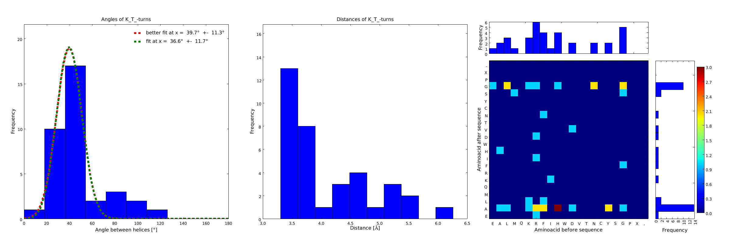
Figure 2) These distributions are subsets of the ones of Figure 1, with only the loops composed of the amino acid T preceded by the amino acid K. This constrain considerably narrows down the angle and length distributions.

Figure 3) Same procedure as in Figure 2. with the loops composed of the amino acid T followed by the amino acid A. This also narrows down the angle and length distributions compared to Figure 1., although not as much as in Figure 2.
Figure 4) The distributions correspond to loops composed of the amino acids KTA and therefore to subsets of all the preceeding ones. One can notice that the angle distribution becomes very narrow, but also that the frequency is reduced compared to the preceeding ones.
This step had two main goals: narrowing down the angle distribution and finding loops with no preferences for the amino acid surrounding them. This last point was important for the modularity of our approach: the angle blocks should not be affected by the surrounding alpha helices. Using this approach, 10 different angle motifs (table 1) could be identified producing different angles. Importantly, all these motifs were chosen so that the length of the two segments starting from the turning point was the same for all of them (put figure turning point). It should also be noticed that 3 of the patterns, KTA, LVA and AAIAP, produce the same angles. There were nevertheless all kept for the in silico refinement described below. But only one was used for the CRAUT software.
| Angle Patterns | |||||||||
|---|---|---|---|---|---|---|---|---|---|
| Pattern | NVL | KTA | LVA | AAIAP | AADGTL | VNLTA | AAAHPEA | ASLPAA | ATGDLA |
| Mean | 29.7 | 38.7 | 35 | 36.5 | 60 | 74.5 | 117 | 140 | 160 |
| Variation | 8.5 | 30 | 29 | 27 | 12 | 27 | 12 | 15 | 5 |
Sequences to connect the alpha helix to the protein extremity
Helical patterns often affect the folding of the attached sequences. To prevent them from affected the structure of the protein of interest, we analyzed the effects of various aminoacids in silico using online tools like pep-fold on helix formation. We identified glycines and prolines as reliable amino acids to interrupt helix formation. We then decided to use glycine pairs to connect the protein of interest to the linker, because they give more flexibility to the initial orientation of the initial helix. This only concerns the protein end that was connected to the linker through the coding sequence. The other end is ligated through exteins or sortase scar, both treated as unstructured flexible regions.
Conclusion
The last three parts show how we could design alpha helix and angle pattern blocks and connect them to each other and to the protein of interest. They provide the material that allowed us to transform a linker defined as a geometrical path into a real amino acid sequence in our software.
Thanks to this we could design linkers to circularize DNMT1 and lysozyme. Additionally it was shown for lysozyme, that a customly tailored linker enhances heat-stability compared to a badly designed linker and even to the flexible linker.
In silico refinement
As some of the interesting patterns could not be found often enough to be statistically significant, we decided to make a further refinement in silico by modeling the structure of proteins with circularizing linkers. To perform this for realistic situations, we selected, from the RCSB database, structures of non-homologous target proteins with extremities that are separated enough to require a linker for circularization. First, the CRAUT software generates possible fitting linkers for various proteins. From these possible linkers, the 100 shortest were taken. Among the 3 possible angle patterns that generate the same angle, the software provides only one. But the linker refinement developed here used the three of them for comparison. We assume that the linkers connect the ends of the protein without setting tension on the protein, so that the protein can fold in its natural way.
After this the circularized proteins with the specific linkers are modelled using a software called Modeller [10]. This software is widely used for comparative structure prediction. It is well established in the scientific community and should be most suitable for prediction of loop regions attached to existing structures [11]. It is freely available for academical usage from the salilab webpages. The program is able to predict the 3d structure of a given sequence based on an alignment with a given structure. In our script Modeller needed to be provided with a sequence with the linker attached and with the PDB file of the protein of interest. This latter file is the only structural information used here. Modeller is recommended when at least 30% sequence similarity exists between the provided structure and the one that the user wish to model. Here, only the linker is different, so this similarity if around 90% in our case. At first Modeller makes an alignment between the provided structure and the sequence of our linked protein, identifying the regions that cannot be found in the structure. Based on that, Modeller generates 4 initial models. One of the strengths of the software is its capacity to further refine only certain parts of the protein. Thus we let Modeller refine the loops, which are defined as any part of the protein that could not be found in the structure file. The ab initio modelling of our linkers is made by minimizing energy functions with different methods like conjugate gradients and molecular dynamics. Eventually, each modeled structure is provided with energy values, thanks to which different models of the same structure can be compared. From Modeller we received about 8 different models and choose the one with the best energy scores to further proceed. For these refinement steps, one can choose different levels of optimization. We always decided for accuracy instead of velocity of the program. The result of a prediction for lysozyme of bacteriophage lambda can be seen in figure 5.
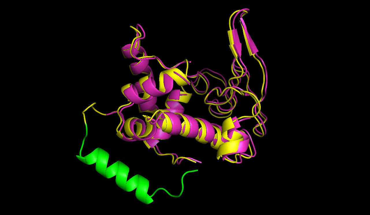
The structure of circular lysozyme (yellow) was predicted and aligned to the linear structure (purple). The linker calculated by the software was marked in green.
Modeller was run by distributing calculation via the iGEM@home system system. The modelling of one linker took about 10 hours of calculation time on average, a value that is highly depending on the size of the protein. Then the best model is evaluated by another self-written program to analyze the behaviour of the linker patterns in their natural surroundings. Finally, all the models for the different structures and the different linkers are analyzed for their properties like the length of the helical patterns, the shape of the attachment structures of the linker and the angles produced by the angle patterns Figure helix_winkel_messung.png. First the modeled structure and the natural structure are fitted, to see how big the differences between those are. If the protein has been disturbed too much, the model is discarded. We control that the alpha helix patterns really generate the expected pattern by measuring the distance between the first and the last amino acids of each of them and checking if it is compatible with an alpha helix. These first and last amino acids of each rods define a vector that is then used to calculate the angles between consecutive helical patterns. The frequency of all the determined lengths and angles is then further analyzed, using a similar strategy to the ArchDB analysis presented above.
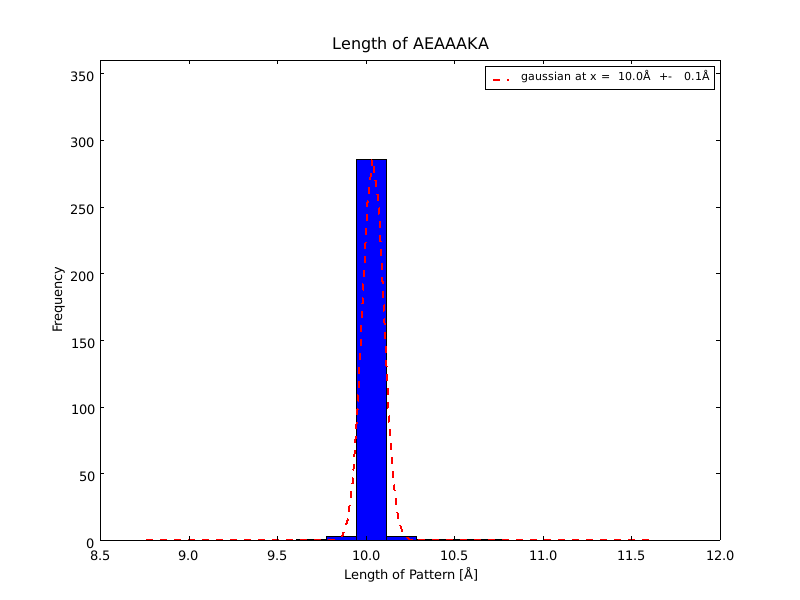
The whole process for the verification of the different linker patterns was set up on the distributed computing system. Due to lack of time, only few results could be analyzed, resulting in distributions for the different helices, see for example figures 6 and 7. This lead to a refinement of the length of the 8 different alpha helix blocks presented above to 8.7, 10, 10.8, 15.6, 16.8, 24.8, 32.3 Å.

Conclusion
The patterns that we identified by analyzing structure databases provide an easy and fast tool to build customly shaped peptides. The main achievement is the identification of the angle patterns. These are designed as building blocks for enhanced applicability. The shapes were identified from a database of non-homologous proteins and the patterns were refined until the distribution of surrounding amino acids looked randomly distributed. Thus we can exclude that the angle distributions we observed is not due to the surrounding sequences, but to the identified patterns. We have not observed any evidence for certain helix patterns being preferred in the database. From figures 6 and 7 we have learned that the lengths we have assumed for the helices needed to be refined. For example we had assumed the AEAAAKA motif to span a distance of 10.5 Å but have observed it to be only 10 Å long. Our CRAUT software was accordingly corrected.
References
[1] Vieille, C. & Zeikus, G.J. Hyperthermophilic enzymes: sources, uses, and molecular mechanisms for thermostability. Microbiology and molecular biology reviews : MMBR 65, 1-43 (2001).
[2] Yu, Y. & Lutz, S. Circular permutation: a different way to engineer enzyme structure and function. Trends Biotechnol. 29, 18-25 (2011).
[3] Arai, R., Ueda, H., Kitayama, a, Kamiya, N. & Nagamune, T. Design of the linkers which effectively separate domains of a bifunctional fusion protein. Protein Eng. 14, 529-532 (2001).
[4] Wang, C.K.L., Kaas, Q., Chiche, L. & Craik, D.J. CyBase: A database of cyclic protein sequences and structures, with applications in protein discovery and engineering. Nucleic Acids Research 36, (2008).
[5] Efimov, a V. Standard structures in proteins. Prog. Biophys. Mol. Biol. 60, 201-2–39 (1993).
[6] Donate, L. E., Rufino, S. D., Canard, L. H. & Blundell, T. L. Conformational analysis and clustering of short and medium size loops connecting regular secondary structures: a database for modeling and prediction. Protein Sci. 5, 2600-26–16 (1996).
[7] Bonet, J. et al. ArchDB 2014: structural classification of loops in proteins. Nucleic Acids Res. 42, D315-D31–9 (2014).
[8] George, R. a & Heringa, J. An analysis of protein domain linkers: their classification and role in protein folding. Protein Eng. 15, 871-879 (2002).
[9] Chen, X., Zaro, J. L. & Shen, W.-C. Fusion protein linkers: property, design and functionality. Adv. Drug Deliv. Rev. 65, 1357-1369 (2013).
[10] Fiser, a et al. Modeling of loops in protein structures. Protein science : a publication of the Protein Society 9, 1753-73 (2000).
[11] Fiser, A. & Sali, A. ModLoop: Automated modeling of loops in protein structures. Bioinformatics 19, 2500-2501 (2003).