 "
"
Team:Freiburg/Content/Results/Modeling
From 2014.igem.org
Lu.jialiang (Talk | contribs) |
Lu.jialiang (Talk | contribs) |
||
| Line 51: | Line 51: | ||
<figure> | <figure> | ||
<a href="https://static.igem.org/mediawiki/2014/6/62/Freiburg2014_Results_modeling_pde.jpg"> <!-- ORGINAL --> | <a href="https://static.igem.org/mediawiki/2014/6/62/Freiburg2014_Results_modeling_pde.jpg"> <!-- ORGINAL --> | ||
| - | <img src="https://static.igem.org/mediawiki/2014/6/62/Freiburg2014_Results_modeling_pde.jpg"> <!-- Thumbnail --> | + | <img style="width: auto;" class="img-no-border" src="https://static.igem.org/mediawiki/2014/6/62/Freiburg2014_Results_modeling_pde.jpg"> <!-- Thumbnail --> |
</a> | </a> | ||
</figure> | </figure> | ||
| Line 60: | Line 60: | ||
<figure> | <figure> | ||
<a href="https://static.igem.org/mediawiki/2014/9/96/Freiburg2014_Results_modeling_D_v.jpg"> <!-- ORGINAL --> | <a href="https://static.igem.org/mediawiki/2014/9/96/Freiburg2014_Results_modeling_D_v.jpg"> <!-- ORGINAL --> | ||
| - | <img src="https://static.igem.org/mediawiki/2014/9/96/Freiburg2014_Results_modeling_D_v.jpg"> <!-- Thumbnail --> | + | <img style="width: auto;" class="img-no-border" src="https://static.igem.org/mediawiki/2014/9/96/Freiburg2014_Results_modeling_D_v.jpg"> <!-- Thumbnail --> |
</a> | </a> | ||
</figure> | </figure> | ||
| Line 69: | Line 69: | ||
<figure> | <figure> | ||
<a href="https://static.igem.org/mediawiki/2014/1/1b/Freiburg2014_Results_modeling_u.jpg"> <!-- ORGINAL --> | <a href="https://static.igem.org/mediawiki/2014/1/1b/Freiburg2014_Results_modeling_u.jpg"> <!-- ORGINAL --> | ||
| - | <img src="https://static.igem.org/mediawiki/2014/1/1b/Freiburg2014_Results_modeling_u.jpg"> <!-- Thumbnail --> | + | <img style="width: auto;" class="img-no-border" src="https://static.igem.org/mediawiki/2014/1/1b/Freiburg2014_Results_modeling_u.jpg"> <!-- Thumbnail --> |
</a> | </a> | ||
</figure> | </figure> | ||
| Line 78: | Line 78: | ||
<figure> | <figure> | ||
<a href="https://static.igem.org/mediawiki/2014/6/68/Freiburg2014_Results_modeling_pdebc2.jpg"> <!-- ORGINAL --> | <a href="https://static.igem.org/mediawiki/2014/6/68/Freiburg2014_Results_modeling_pdebc2.jpg"> <!-- ORGINAL --> | ||
| - | <img src="https://static.igem.org/mediawiki/2014/6/68/Freiburg2014_Results_modeling_pdebc2.jpg"> <!-- Thumbnail --> | + | <img style="width: auto;" class="img-no-border" src="https://static.igem.org/mediawiki/2014/6/68/Freiburg2014_Results_modeling_pdebc2.jpg"> <!-- Thumbnail --> |
</a> | </a> | ||
</figure> | </figure> | ||
| Line 87: | Line 87: | ||
<figure> | <figure> | ||
<a href="https://static.igem.org/mediawiki/2014/0/0b/Freiburg2014_Results_modeling_pdebc1.jpg"> <!-- ORGINAL --> | <a href="https://static.igem.org/mediawiki/2014/0/0b/Freiburg2014_Results_modeling_pdebc1.jpg"> <!-- ORGINAL --> | ||
| - | <img src="https://static.igem.org/mediawiki/2014/0/0b/Freiburg2014_Results_modeling_pdebc1.jpg"> <!-- Thumbnail --> | + | <img style="width: auto;" class="img-no-border" src="https://static.igem.org/mediawiki/2014/0/0b/Freiburg2014_Results_modeling_pdebc1.jpg"> <!-- Thumbnail --> |
</a> | </a> | ||
</figure> | </figure> | ||
| Line 122: | Line 122: | ||
<figure> | <figure> | ||
<a href="https://static.igem.org/mediawiki/2014/3/3c/Freiburg2014_Results_modeling_Cf.jpg"> <!-- ORGINAL --> | <a href="https://static.igem.org/mediawiki/2014/3/3c/Freiburg2014_Results_modeling_Cf.jpg"> <!-- ORGINAL --> | ||
| - | <img src="https://static.igem.org/mediawiki/2014/3/3c/Freiburg2014_Results_modeling_Cf.jpg"> <!-- Thumbnail --> | + | <img style="width: auto;" class="img-no-border" src="https://static.igem.org/mediawiki/2014/3/3c/Freiburg2014_Results_modeling_Cf.jpg"> <!-- Thumbnail --> |
</a> | </a> | ||
</figure> | </figure> | ||
<figure> | <figure> | ||
<a href="https://static.igem.org/mediawiki/2014/d/d7/Freiburg2014_Results_modeling_Cc.jpg"> <!-- ORGINAL --> | <a href="https://static.igem.org/mediawiki/2014/d/d7/Freiburg2014_Results_modeling_Cc.jpg"> <!-- ORGINAL --> | ||
| - | <img src="https://static.igem.org/mediawiki/2014/d/d7/Freiburg2014_Results_modeling_Cc.jpg"> <!-- Thumbnail --> | + | <img style="width: auto;" class="img-no-border" src="https://static.igem.org/mediawiki/2014/d/d7/Freiburg2014_Results_modeling_Cc.jpg"> <!-- Thumbnail --> |
</a> | </a> | ||
</figure> | </figure> | ||
<figure> | <figure> | ||
<a href="https://static.igem.org/mediawiki/2014/2/2c/Freiburg2014_Results_modeling_Ci.jpg"> <!-- ORGINAL --> | <a href="https://static.igem.org/mediawiki/2014/2/2c/Freiburg2014_Results_modeling_Ci.jpg"> <!-- ORGINAL --> | ||
| - | <img src="https://static.igem.org/mediawiki/2014/2/2c/Freiburg2014_Results_modeling_Ci.jpg"> <!-- Thumbnail --> | + | <img style="width: auto;" class="img-no-border" src="https://static.igem.org/mediawiki/2014/2/2c/Freiburg2014_Results_modeling_Ci.jpg"> <!-- Thumbnail --> |
</a> | </a> | ||
</figure> | </figure> | ||
<figure> | <figure> | ||
<a href="https://static.igem.org/mediawiki/2014/3/30/Freiburg2014_Results_modeling_Vf.jpg"> <!-- ORGINAL --> | <a href="https://static.igem.org/mediawiki/2014/3/30/Freiburg2014_Results_modeling_Vf.jpg"> <!-- ORGINAL --> | ||
| - | <img src="https://static.igem.org/mediawiki/2014/3/30/Freiburg2014_Results_modeling_Vf.jpg"> <!-- Thumbnail --> | + | <img style="width: auto;" class="img-no-border" src="https://static.igem.org/mediawiki/2014/3/30/Freiburg2014_Results_modeling_Vf.jpg"> <!-- Thumbnail --> |
</a> | </a> | ||
</figure> | </figure> | ||
<figure> | <figure> | ||
<a href="https://static.igem.org/mediawiki/2014/6/6e/Freiburg2014_Results_modeling_Vc.jpg"> <!-- ORGINAL --> | <a href="https://static.igem.org/mediawiki/2014/6/6e/Freiburg2014_Results_modeling_Vc.jpg"> <!-- ORGINAL --> | ||
| - | <img src="https://static.igem.org/mediawiki/2014/6/6e/Freiburg2014_Results_modeling_Vc.jpg"> <!-- Thumbnail --> | + | <img style="width: auto;" class="img-no-border" src="https://static.igem.org/mediawiki/2014/6/6e/Freiburg2014_Results_modeling_Vc.jpg"> <!-- Thumbnail --> |
</a> | </a> | ||
</figure> | </figure> | ||
<figure> | <figure> | ||
<a href="https://static.igem.org/mediawiki/2014/c/cb/Freiburg2014_Results_modeling_Vi.jpg"> <!-- ORGINAL --> | <a href="https://static.igem.org/mediawiki/2014/c/cb/Freiburg2014_Results_modeling_Vi.jpg"> <!-- ORGINAL --> | ||
| - | <img src="https://static.igem.org/mediawiki/2014/c/cb/Freiburg2014_Results_modeling_Vi.jpg"> <!-- Thumbnail --> | + | <img style="width: auto;" class="img-no-border" src="https://static.igem.org/mediawiki/2014/c/cb/Freiburg2014_Results_modeling_Vi.jpg"> <!-- Thumbnail --> |
</a> | </a> | ||
</figure> | </figure> | ||
| Line 155: | Line 155: | ||
<figure> | <figure> | ||
<a href="https://static.igem.org/mediawiki/2014/0/02/Freiburg2014_Results_modeling_delta1.jpg"> <!-- ORGINAL --> | <a href="https://static.igem.org/mediawiki/2014/0/02/Freiburg2014_Results_modeling_delta1.jpg"> <!-- ORGINAL --> | ||
| - | <img src="https://static.igem.org/mediawiki/2014/0/02/Freiburg2014_Results_modeling_delta1.jpg"> <!-- Thumbnail --> | + | <img style="width: auto;" class="img-no-border" src="https://static.igem.org/mediawiki/2014/0/02/Freiburg2014_Results_modeling_delta1.jpg"> <!-- Thumbnail --> |
</a> | </a> | ||
</figure> | </figure> | ||
| Line 163: | Line 163: | ||
<figure> | <figure> | ||
<a href="https://static.igem.org/mediawiki/2014/7/7a/Freiburg2014_Results_modeling_nv.jpg"> <!-- ORGINAL --> | <a href="https://static.igem.org/mediawiki/2014/7/7a/Freiburg2014_Results_modeling_nv.jpg"> <!-- ORGINAL --> | ||
| - | <img src="https://static.igem.org/mediawiki/2014/7/7a/Freiburg2014_Results_modeling_nv.jpg"> <!-- Thumbnail --> | + | <img style="width: auto;" class="img-no-border" src="https://static.igem.org/mediawiki/2014/7/7a/Freiburg2014_Results_modeling_nv.jpg"> <!-- Thumbnail --> |
</a> | </a> | ||
</figure> | </figure> | ||
| Line 175: | Line 175: | ||
<figure> | <figure> | ||
<a href="https://static.igem.org/mediawiki/2014/f/f1/Freiburg2014_Results_modeling_eff.jpg"> <!-- ORGINAL --> | <a href="https://static.igem.org/mediawiki/2014/f/f1/Freiburg2014_Results_modeling_eff.jpg"> <!-- ORGINAL --> | ||
| - | <img src="https://static.igem.org/mediawiki/2014/f/f1/Freiburg2014_Results_modeling_eff.jpg"> <!-- Thumbnail --> | + | <img style="width: auto;" class="img-no-border" src="https://static.igem.org/mediawiki/2014/f/f1/Freiburg2014_Results_modeling_eff.jpg"> <!-- Thumbnail --> |
</a> | </a> | ||
</figure> | </figure> | ||
| Line 191: | Line 191: | ||
<figure> | <figure> | ||
<a href="https://static.igem.org/mediawiki/2014/1/1f/Freiburg2014_Results_modeling_exp_decay.jpg"> <!-- ORGINAL --> | <a href="https://static.igem.org/mediawiki/2014/1/1f/Freiburg2014_Results_modeling_exp_decay.jpg"> <!-- ORGINAL --> | ||
| - | <img src="https://static.igem.org/mediawiki/2014/1/1f/Freiburg2014_Results_modeling_exp_decay.jpg"> <!-- Thumbnail --> | + | <img style="width: auto;" class="img-no-border" src="https://static.igem.org/mediawiki/2014/1/1f/Freiburg2014_Results_modeling_exp_decay.jpg"> <!-- Thumbnail --> |
</a> | </a> | ||
</figure> | </figure> | ||
| Line 204: | Line 204: | ||
<p class="header"><b>Figure 5. </b> Extracellular degradation of MLV. MLV vectors were incubated in cell-free medium at 37 °C for different duration and then infected NIH-3T3 cells for 72h. Transduction efficiency was measured by FACS. A single exponential function was fitted to the data (shown in line).</p> | <p class="header"><b>Figure 5. </b> Extracellular degradation of MLV. MLV vectors were incubated in cell-free medium at 37 °C for different duration and then infected NIH-3T3 cells for 72h. Transduction efficiency was measured by FACS. A single exponential function was fitted to the data (shown in line).</p> | ||
</figcaption> | </figcaption> | ||
| - | + | </figure> | |
| - | <p>The extracellular degradation rate was about 0.124 and the half-life of MLV equals 5.6 h. This result is in good consistent with that obtained by Tayi et al. and shows the instability of the retroviral vector at physiological temperature in extracellular conditions. </p> | + | <p>The extracellular degradation rate was about 0.124 h<sup>-1</sup> and the half-life of MLV equals 5.6 h. This result is in good consistent with that obtained by Tayi et al. and shows the instability of the retroviral vector at physiological temperature in extracellular conditions. </p> |
<h3>Estimation of viral titer</h3> | <h3>Estimation of viral titer</h3> | ||
| + | <p>Due to limited time, we did not carry out all experiments to determine every parameter. Thus the remaining parameters including binding, intracellular degradation, integration rate and trafficking time were adopted from Tayi’s paper. By means of this model with the parameter, we estimated the viral titer of our MLV suspension. </p> | ||
| + | <p>In this case, mouse cells were infected by MLV for different durations and then incubated in virus-free medium for a certain time. The equations with an unknown virus concentration were solved and fitted to the experimental data using least square estimation (see Fig. 6). </p> | ||
| + | <figure> | ||
| + | <a href="https://static.igem.org/mediawiki/2014/2/24/Freiburg2014_Results_modeling_integration.jpg"> <!-- ORGINAL --> | ||
| + | <img src="https://static.igem.org/mediawiki/2014/2/24/Freiburg2014_Results_modeling_integration.jpg"> <!-- Thumbnail --> | ||
| + | </a> | ||
| + | <figcaption> | ||
| + | <p class="header"><b>Figure 6. </b> Extracellular degradation of MLV. MLV vectors were incubated in cell-free medium at 37 °C for different duration and then infected NIH-3T3 cells for 72h. Transduction efficiency was measured by FACS. A single exponential function was fitted to the data (shown in line).</p> | ||
| + | </figcaption> | ||
| + | </figure> | ||
| + | <p>The virus titer is 1.2∙10<sup>7</sup> vectors/ml. This value is typical for standard protocols with helper-free retroviral production. </p> | ||
| + | <h3>Verification of virus titer</h3> | ||
| + | <p>The estimated virus titer was verified by predicting the transduction efficiency with virus dilution and comparing it with the experimental data. MLV stock was diluted with a factor 0.1 to 0.5 and incubated with mouse cells. Transduction efficiency measured at the end of the experiments was shown in Fig. 7 as well as the prediction from our model. </p> | ||
| + | <figure> | ||
| + | <a href="https://static.igem.org/mediawiki/2014/1/1f/Freiburg2014_Results_modeling_dilution.jpg"> <!-- ORGINAL --> | ||
| + | <img src="https://static.igem.org/mediawiki/2014/1/1f/Freiburg2014_Results_modeling_dilution.jpg"> <!-- Thumbnail --> | ||
| + | </a> | ||
| + | <figcaption> | ||
| + | <p class="header"><b>Figure 7. </b> Verification of virus titer. MLV suspension was diluted by different factors and added to the cells and incubated for 48 h. The viral titre estimated in the last experiments was used to predict the transduction efficiency (shown in line). </p> | ||
| + | </figcaption> | ||
| + | </figure> | ||
| - | + | <p>The prediction was consistent with the data. The result demonstrated that our model was a good simulation of the infection process and could be applied for further experiments. </p> | |
| - | + | ||
| - | + | ||
| - | + | ||
| - | + | ||
</section> | </section> | ||
| Line 229: | Line 246: | ||
</section> | </section> | ||
| + | <!-- ===================================================Light model=================================================== --> | ||
<section> | <section> | ||
<h2 id="Results-Modeling-Light-System-Model-Formulation">Model Formulation</h2> | <h2 id="Results-Modeling-Light-System-Model-Formulation">Model Formulation</h2> | ||
Revision as of 20:24, 16 October 2014
Modeling
The AcCELLerator is based on the combination of two systems: the light-regulated gene expression and the retroviral gene delivery.
MLV Infection
Model Formulation
In our project, gene delivery was achieved by infecting the cells with recombinant murine leukemia virus (MLV). As a typical retrovirus, its life cycle has been well characterized. Usually, this process can be divided artificially into several steps, including adsorption, internalization, integration, replication, assembly and release. However, our recombinant MLVs lacked the genes which are essentially for the replication and the virus assembly. Thus only the gene of interest (GOI) could be integrated into the genome and expressed. The process from adsorption to integration can be again subdivided into seven steps, so that each step can be described with a simple mathematical model.

Figure 1. (1) The infection is initiated by the adsorption of the virions onto the cell surface, which is covered by the specific receptor mCAT1. (2) Once the virion binds with the receptor, fusion of viral and cell membrane is triggered and the viral core is internalized into the cytoplasm. (3) Using viral RNA as template, double stranded DNA is produced by reverse transcriptase. (4) The viral DNA is then transported along the microtubuli to the microtubule organizing center near the nucleus. (5) During the transcription and transport, the viral molecules could be degraded by cellular factors. (6) During cell division, the nuclear envelope dissolves and the viral DNA is imported into the nucleus. (7) Viral DNA is integrated into the chromosome by integrase. (modified from1)
The whole infection process was described by a set of differential equations, which was adopted from a previous work1 with small modifications.
First, a viral suspension of depth h was added to a layer of adherent cells to infect them (see Fig. 2). The concentration of the virion (Vm) is a function of both time and depth. It is influenced by four different processes: diffusion, sedimentation, degradation and binding.

Figure 2. Virus suspension and cells
The diffusion of the virions follows the fick’s law of diffusion. u is the velocity of sedimentation due to gravity. Since the virions are instable at 37°C, they decay in the medium with a constant decay rate kd_vm. Thus an additional term was added to the partial differential equation (PDE).

The diffusion coefficient Dv can be calculated according to the Stokes–Einstein equation,

and u was estimated as the Stokes settling velocity.

To solve the PDE, boundary conditions are required at the top and the bottom of the medium. At the top (z=h), net flux of virions has to be zero, so that

At the bottom (z=0), virions bind irreversibly onto the cell surface and are subsequently internalized. The binding rate is proportional to local virus concentration, cell density and density of mCAT1 receptor on the cell surface. Moreover, the binding is saturating at high receptor density, so a Michaelis-constant for receptor density was added to the equation.

Second, the MLV undergoes several steps (see Fig. 1 (3)-(7)) after the internalization to be integrated into the genome. However, it is difficult to determine the intracellular concentration of each viral component. The only output of our experiments was the transduction efficiency determined by flow cytometry. Thus it makes more sense to consider the dynamics between infected and non-infected cells.
According to the location of intracellular viral particles, the cells were divided into three populations (see Fig. 3): virus-free cells (Cf), cells that carry MLV in the cytoplasm (Cc) and cells with viral DNA integrated in the genome (Ci). Similarly, intracellular viral particles were divided into cytoplasmic viruses (Vc) and integrated viruses (Vi). Particularly, a subpopulation of cytoplasmic virus inside the virus-carrying cells only (Vf) was also considered to enable further calculations.

Figure 3. Cell and virus populations and their density.
The dynamics between different cell and virus populations was influenced by several factors (see Fig. 4), including binding of new virions, intracellular degradation of viral particles wit rate kd_vc, integration of viral DNA with integration rate kin, and cell division with a constant growth rate μ.
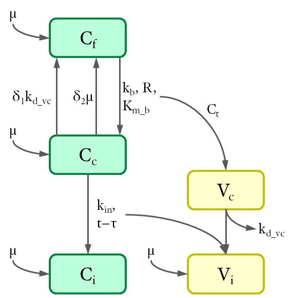
Figure 4. Dynamics of cell and virus populations.
Thus the differential equations were set up as follows.


δ1 is the possibility of a virus-carrying cell that becomes virus-free owing to the degradation of intracellular virus. Since multiple cytoplasmic viruses are unlikely to degrade at the same time, the possibility equals the fraction of virus-carrying cells with only one virus. Since the distribution of the multiplicities of infection (MOI) follows the poisson distribution, δ1 can be calculated using the following equation,

where n_v is the average number of virus per cell inside the virus-carrying cells.

δ2 is the possibility of a virus-carrying cell that becomes virus-free during cell division. Because virus particles enter two daughter cells in a random process, one of them may lose all particles and became virus-free again. δ2 depends on the MOI of the cell.
Besides, terms for the integration are calculated at time τ prior to the current time point t. τ is the mean trafficking time of the virus inside the cytoplasm and includes time for reverse transcription and viral transport (see Fig. 1 (3)-(4)). These terms turn these differential equations into a delayed differential equation system (DDE), which was solved here by numerical methods using MATLAB.
The experimental output, the transduction efficiency, is defined as the fraction of virus-integrated cells.

Data Analysis
Extracellular virus degradation
The extracellular degradation rate of MLV (kd_vm) was first investigated. MLV suspension was incubated at 37 °C for different durations. The viral concentration should follow a single exponential decay function.

In our experiment, the virus suspension was transferred to the cells after the incubation and transduction efficiency was measured. The results was fitted to an exponential function to determine the degradation rate (see Fig. 5).

Figure 5. Extracellular degradation of MLV. MLV vectors were incubated in cell-free medium at 37 °C for different duration and then infected NIH-3T3 cells for 72h. Transduction efficiency was measured by FACS. A single exponential function was fitted to the data (shown in line).
The extracellular degradation rate was about 0.124 h-1 and the half-life of MLV equals 5.6 h. This result is in good consistent with that obtained by Tayi et al. and shows the instability of the retroviral vector at physiological temperature in extracellular conditions.
Estimation of viral titer
Due to limited time, we did not carry out all experiments to determine every parameter. Thus the remaining parameters including binding, intracellular degradation, integration rate and trafficking time were adopted from Tayi’s paper. By means of this model with the parameter, we estimated the viral titer of our MLV suspension.
In this case, mouse cells were infected by MLV for different durations and then incubated in virus-free medium for a certain time. The equations with an unknown virus concentration were solved and fitted to the experimental data using least square estimation (see Fig. 6).
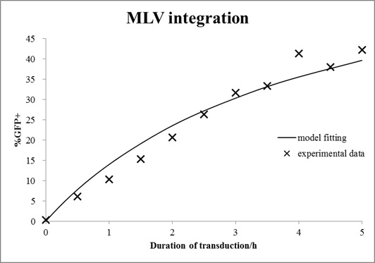
Figure 6. Extracellular degradation of MLV. MLV vectors were incubated in cell-free medium at 37 °C for different duration and then infected NIH-3T3 cells for 72h. Transduction efficiency was measured by FACS. A single exponential function was fitted to the data (shown in line).
The virus titer is 1.2∙107 vectors/ml. This value is typical for standard protocols with helper-free retroviral production.
Verification of virus titer
The estimated virus titer was verified by predicting the transduction efficiency with virus dilution and comparing it with the experimental data. MLV stock was diluted with a factor 0.1 to 0.5 and incubated with mouse cells. Transduction efficiency measured at the end of the experiments was shown in Fig. 7 as well as the prediction from our model.

Figure 7. Verification of virus titer. MLV suspension was diluted by different factors and added to the cells and incubated for 48 h. The viral titre estimated in the last experiments was used to predict the transduction efficiency (shown in line).
The prediction was consistent with the data. The result demonstrated that our model was a good simulation of the infection process and could be applied for further experiments.